Ecosystems and Human Well-Being: Volume 1: Current State and Trends: Biodiversity

Published: March 15, 2009, 2:00 pm

Updated: September 7, 2011, 6:47 am

Source: Millennium Ecosystem Assessment

Topics:

Human Health (main) Environmental Monitoring (main) Biodiversity (main) Environmental Assessment (main) Ecology (main) International Environmental Issues (main)

This is Chapter 4 of the Millenium Ecosystem Assessment report Ecosystems and Human Well-Being: Volume 1: Current State and Trends

Coordinating Lead Authors: Georgina Mace, Hillary Masundire, Jonathan Baillie
Lead Authors: Taylor Ricketts, Thomas Brooks, Michael Hoffmann, Simon Stuart, Andrew Balmford, Andy Purvis, Belinda Reyers, Jinliang Wang, Carmen Revenga, Elizabeth Kennedy, Shahid Naeem, Rob Alkemade, Tom Allnutt, Mohamed Bakarr, William Bond, Janice Chanson, Neil Cox, Gustavo Fonseca, Craig Hilton-Taylor, Colby Loucks, Ana Rodrigues, Wes Sechrest, Alison Stattersfield, Berndt Janse van Rensburg, Christina Whiteman
Contributing Authors: Robin Abell, Zoe Cokeliss, John Lamoreux, Henrique Miguel Pereira, Jillian Thönell, Paul Williams
Review Editors: Gerardo Ceballos, Sandra Lavorel, Gordon Orians, Steve Pacala

Main Messages

Biodiversity—the diversity of genes, populations, species (Species diversity), communities, and ecosystems—underlies all ecosystem processes. Ecological processes interacting with the atmosphere, geosphere, and hydrosphere determine the environment on which organisms, including people, depend. Direct benefits such as food crops, clean water, clean air, and aesthetic pleasures all depend on biodiversity, as does the persistence, stability, and productivity of natural systems.

For many ecosystem services, local population extinctions are more significant than global extinctions—human communities depend for their well-being on populations of species that are accessible to them. The most appropriate measures and indicators of biodiversity depend on the value or service being assessed and involve a consideration of the components of biodiversity that are involved (from genes, individuals, populations, species, and communities to ecosystems) and the service that is being delivered.

Knowledge of biodiversity is uneven, with strong biases toward the species level, large animals, temperate systems, and components of biodiversity used by people. This results in gaps in knowledge, especially regarding the status of tropical systems, marine and freshwater biota, plants, invertebrates, microorganisms, and subterranean biota.

Most estimates of the total number of species on Earth lie between 5 million and 30 million. Of this total, roughly 2 million species have been formally described; the remainder are unknown or unnamed. The overall total could be higher than 30 million if poorly known groups such as deep-sea organisms, fungi, and microorganisms including parasites have more species than currently estimated.

Most macroscopic organisms have small, often clustered, geographical ranges, leading to diagnosable centers of both diversity and endemism, which are frequently concentrated in isolated or topographically variable regions (islands, mountains, peninsulas). A large proportion of the world’s terrestrial biodiversity at the species level is concentrated in a small area of the world, mostly in the tropics. The Neotropics and Afrotropics have the highest species richness. Endemism is also high in these regions and, as a consequence of its isolation, in Australasia. Even among the larger and more mobile species such as the terrestrial vertebrates, more than one third of all species have ranges less than 1,000 square kilometers. In contrast, local and regional diversity of microorganisms appears to be more similar to large-scale and global diversity, indicating greater dispersal, larger range sizes, and lower levels of regional species clustering.

Across a range of measures, tropical forests are outstanding in their levels of biodiversity at and above the species level. Regions of high species richness broadly correspond with centers of evolutionary diversity, and available evidence suggests that across major taxa, tropical moist forests are especially important for both overall variability and unique evolutionary history. Species richness, family richness, and species endemism are all highest for this biome, even after accounting for area and productivity.

Over the past few hundred years humans may have increased the species extinction rate by as much as three orders of magnitude. This estimate is uncertain because the extent of extinctions in undescribed taxa is unknown, because the status of many described species is poorly known, because it is difficult to document the final disappearance of very rare species, and because there are extinction lags between the impact of a threatening process and the resulting extinction. However, the most definite information, based on recorded extinctions of known species over the past 100 years, indicates extinction rates are around 100 times greater than rates characteristic of species in the fossil record. Other less direct estimates, some of which refer to extinctions hundreds of years into the future, estimate extinction rates 1,000 to 10,000 times higher than rates recorded among fossil lineages.

Between 12% and 52% of species within well-studied higher taxa are threatened with extinction, according to the IUCN Red List. Less than 10% of named species have been assessed in terms of their conservation status. Of those that have, birds have the lowest percentage of threatened species at 12%. The patterns of threat are broadly similar for mammals and conifers, which have 23% and 25% of species threatened, respectively. The situation with amphibians looks similar, with 32% threatened, but information is more limited. so this may be an underestimate. Cycads have a much higher proportion of threatened species, with 52% globally threatened. In regional assessments, taxonomic groups with the highest proportion of threatened species tended to be those that rely on freshwater (Freshwater biomes) habitats. Threatened species show continuing declines in conservation status, and species threat rates tend to be highest in the realms with highest species richness.

The main causes of species extinction are changing from a historical trend of introductions and overexploitation affecting island species to present-day habitat loss and degradation affecting continental species. While the vast majority of recorded extinctions since 1500 have occurred on oceanic islands, continental extinctions are now as common as island extinctions. Approximately 50% of extinctions over the past 20 years occurred on continents. This trend is consistent with the observation that most terrestrial species threatened with extinction are continental. Despite the growing importance of habitat loss and degradation, species introductions and overexploitation also remain significant threats to biodiversity on continents and islands.

Climate change, which contributes to habitat change, is becoming the dominant driver, particularly in vulnerable habitats. Under climate change, endemic montane, island, and peninsula species are especially vulnerable, and coastal habitats such as mangroves, coral reefs, and coastal wetlands are especially at risk from resulting sea level rises. Both recent empirical evidence and predictive modeling studies suggest that climate change will increase population losses. In some regions there may be an increase in local biodiversity— usually as a result of species introductions, the long-term consequences of which are hard to foresee.

Among a range of higher taxa, the majority of species are currently in decline. Studies of amphibians globally, African mammals, birds in intensively managed agricultural lands, British butterflies, Caribbean corals, waterbirds, and fishery (Fisheries and aquaculture) species show the majority of species to be declining in range or number. Those species that are increasing have benefited from management interventions such as protection in reserves or elimination of threats such as overexploitation or are species that tend to thrive in human-dominated landscapes.

The majority of [[biome]s] have been greatly modified by humans. Between 20% and 50% of 9 of the 14 biomes have been transformed to croplands. Tropical dry forests are the most reduced by cultivation, with almost half of the biome’s native habitats replaced with cultivated lands. Three other biomes— temperate grasslands, temperate broadleaf forests, and Mediterranean forests— have experienced 35% or more conversion. Biomes least reduced by cultivation include deserts, boreal forests (Forest biome), and tundra. While cultivated lands provide many provisioning services, such as grains, fruits, and meat, habitat conversion to agriculture typically leads to reductions in native biodiversity.

Homogenization, the process whereby species assemblages become increasingly dominated by a small number of widespread, human-adapted species, represents further losses in biodiversity that are often missed when only considering changes in absolute numbers of species. The many species that are declining as a result of human activities tend to be replaced by a much smaller number of expanding species that thrive in human-altered environments.

We lack comprehensive global-scale measures to assess whether the internationally agreed target of significantly reducing the rate of loss of biodiversity by 2010 will be met. However, our understanding of the dynamics of drivers, and particularly of lag times from changes in drivers to eventual impacts on biodiversity, suggest it is most unlikely to be achievable. The 2010 target, as agreed at WSSD in 2002 and adopted by the parties to the Convention on Biological Diversity, is an important goal for biodiversity management. It is probably too late to reverse the near-term trends in biodiversity loss given the lag times in ecosystem responses. Until critical drivers are mitigated, most declines seem likely to continue at the same or increased rates, although there is evidence that biodiversity loss is slowing or even recovering for some habitats (such as temperate woodlands) and species (temperate birds, for example).

4.1 Introduction

Biodiversity is fundamental to ecosystem functioning. Extrinsic or abiotic factors, such as climate and geophysical conditions, help to determine the boundaries of ecosystems (Colwell and Lees 2000; Gaston 2000). But within these boundaries, intrinsic or biotic factors such as the abundance, distribution, dynamics, and functional variation among biodiversity components of ecosystems regulate the magnitude and variability of ecosystem processes, such as production or decomposition. (See Chapter 11.) Together, these extrinsic and intrinsic factors determine the specific properties of an ecosystem, such as its stability, its fertility, or its susceptibility to invasion. They also determine the type of ecosystem found, such as drylands, forest or woodland, or inland waters.

The benefits that humans derive from ecosystems are known as ecosystem services (see Chapter 1 (Ecosystems and Human Well-Being: Volume 1: Current State and Trends: Biodiversity)) and include breathable air, fertile soils, and productive forests and fisheries (Fisheries and aquaculture), as well as many cultural benefits such as recreational hunting or inspirational values. Such ecosystem services are obtained only if ecosystems include the biodiversity that guarantees the functional processes necessary to deliver them.

This chapter focuses on the fundamental aspects of biodiversity that underpin all ecosystem processes and that are valued in their own right. Biodiversity relevant to particular services is documented in the Chapters 7 to 17 of this volume, while biodiversity as one element in the management of particular ecosystems for the delivery of services is discussed in Chapters 18 to 27. This chapter describes what is known about biodiversity globally, the nature of biodiversity variation and its measurement, the main drivers of change, and the observed trends in distribution, variation, and abundance of biodiversity.

4.1.1 Biodiversity and Its Assessment

Biodiversity is the diversity among living organisms in terrestrial, marine, and other aquatic ecosystems and the ecological complexes of which they are part. It includes diversity within and between species and the diversity of ecosystems. In addition to the important role of biodiversity in providing ecosystem services, it also has intrinsic value, independent of any human concern.

In addition to its intrinsic value, the roles of biodiversity in the provision of ecosystem services can be summarized under the following headings:

•  ?supporting roles include the underpinning of ecosystems through structural, compositional, and functional diversity;
•  ?regulatory roles through the influence of biodiversity on the production, stability, and resilience of ecosystems;
•  ?cultural roles from the nonmaterial benefits people derive from the aesthetic, spiritual, and recreational elements of biodiversity; and
•  ?provisioning roles from the direct and indirect supply of food, fresh water, fiber, and so on.

All these roles are strongly interrelated, and it is rarely possible to separate them in practice. Yet defining roles is an essential step in assessing biodiversity: any measures should be relevant to the role being examined and to the purpose of the assessment (The Royal Society 2003). For example, a biologist wishing to assess the changing status of biodiversity in a wetland before and after land use changes in the watershed might turn to the most widely available information—trends in bird population sizes. People interested in birds would regard this as important, but if the observer were concerned about overall species richness, the bird data could be insufficient or even misleading. Due to their unusual dispersal ability, birds might be relatively well buffered from the effects of habitat change. The consequences of the land use change on less vagile species, such as plants, invertebrates, or below-ground biota could be very different. Similarly, if the effect on ecosystem services were of most interest, then other species and measures other than population size will be more informative. If provisioning services were under examination, then the assessment would be better focused on the abundance and distribution of the ecosystem components essential for food or fiber production. Thus, given the complexity of biodiversity, the most readily available measures rarely reflect the real attribute of interest for any particular role (The Royal Society 2003).

Biodiversity is commonly measured at the levels of genes, species or ecosystems. At each of these, measures may represent one or many of the following:

• Variety, reflecting the number of different types. For example, this could refer to different species or genes, such as how many bird species live in a particular place or how many varieties of a genetic crop strain are in production.
• Quantity and quality, reflecting how much there is of any one type. Variation on its own will only rarely meet people’s needs. For example, for many provisioning services (food, fresh water, fiber) the quantity or the quality matter more than the presence of a particular genetic variety, species, or ecosystem.
• Distribution, reflecting where that attribute of biodiversity is located. For example, having all the world’s pollinators present but only in a single location will not meet the needs of the plants that depend on them. Many ecosystem services are location-specific. For instance, human and natural communities need to be close to wetlands to benefit from their regulatory roles.

In practice, the relevant measure and attribute depends on the role being assessed. For example, many benefits of biodiversity depend on the functional and structural variability in species, whereas most provisioning services and many regulatory services depend more on the quantity and distribution of populations and ecosystems. Long-term sustainability of many services depends on the maintenance of genetic variability. Ultimately, maintaining variability in any biodiversity component provides options for the future, even if not all variants have an obvious role to play. Thus, variability plays a special role, which probably explains why it is generally emphasized in discussions of biodiversity value.

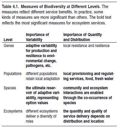
Table 4.1 summarizes the importance of quantity versus variability among different biodiversity components in relation to ecosystem services. Broadly speaking, and according to our present level of understanding, variability is more significant at the genetic and species levels, whereas quantity and distribution are more significant at the population and ecosystem levels. For most ecosystem services, local loss of biodiversity (population reduction or local extinction) is most significant; but for future option values and for certain services such as genetic variability and bioprospecting, global loss is the primary consideration.

4.1.2 The Diversity and Evolution of Life

Living organisms were originally divided into two kingdoms: animal and vegetable (the Animalia and the Plantae), but more recently it has become clear that this simple division does not reflect the true diversity of life. The five Kingdom scheme that followed divided all living organisms into Monera (bacteria), Protista (single-celled organisms), Fungi, Plants, and Animals. In terms of either numerical diversity or phylogenetic diversity (measuring the degree of independent evolutionary history), however, it is now clear that this too misrepresents the diversity of life.

Most organisms are very small (microscopic), and DNA and RNA studies reveal that the living world is more appropriately divided into three groups: the Bacteria, the Archaea (a group once included with the bacteria but now shown to be as different from them as they both are from the rest), and the rest—the Eukaryotae. Bacteria and Archaea have no well-defined nucleus and are referred to as Prokaryotae (or prokaryotes). The Eukaryotae (or eukaryotes) have a well-defined nucleus and comprise the animals, plants, fungi, and protists. A fourth group of biological entities, the viruses, are not organisms in the same sense that eukaryotes, archaeans, and bacteria are, and so they are not included. However, they are of considerable biological importance.

Life arose on Earth 3.5–4.5 billion years ago, and for probably the first 1–2 billion years there were only prokaryotes. The first definitive fossils of eukaryotes are found about 2 billion years ago, but they started to proliferate quite rapidly and the multicellular eukaryotes appear about 1.5 billion years ago. The first animals appeared much later, around 700 million years ago for many soft-bodied marine invertebrates, such as the sponges, jellyfish, soft corals, and worms. By about 500 million years ago an abundant fossil record includes marine invertebrates with exoskeletons, vertebrates, and plants. All phyla existing today appear shortly after. Today’s diverse assemblage of mammals, birds, and flowering plants appeared within the past 70 million years, but it is not until about 7 million years ago that humans in their most primitive form appeared, and not until 100,000–200,000 years ago that modern humans appeared.

Evolutionary biologists believe that all existing life is derived from a single, common ancestral form. The fact that millions of species live on Earth today is a consequence of processes leading to speciation. Speciation involves the splitting of a single species lineage. It occurs in three different ways: allopatric, parapatric, and sympatric. Allopatric speciation is speciation by geographic isolation and requires the imposition of a barrier that prevents individuals in the two lineages from interbreeding with one another. For most animals, geographical isolation has been the most important barrier, and the larger and more vagile the animal, the wider the barrier must be. As a result, allopatric speciation in most animals can take place only in large geographic areas where substantial barriers, such as wide water gaps or isolated mountains exist. In parapatric speciation there is no complete geographic isolation, but lineages diverge across environmental gradients. Sympatric speciation is speciation without geographic isolation. Plants, for example, commonly speciate via a duplication of their chromosomes, a process that can be accomplished in a single generation. The different process and conditions required for speciation results in a great variation in the rate of speciation. However, in general the process is slow, usually taking millions of years.

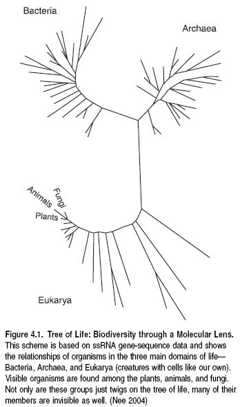
The short and clustered branches on the molecular tree of life (see Figure 4.1) illustrate the relatively close and recent relationships among the organisms with which we are most familiar and that dominate most biodiversity assessments (Plants, Animals, Fungi). However, the microorganisms that dominate the branches of the evolutionary tree are extremely important in any assessment of biodiversity. These groups include most of the forms that are the main providers of most regulating and supporting services and that are key to many provisioning services (Nee 2004).

4.1.3 Practical Issues for Ecosystem Assessment

The term ecosystem can be applied to any functioning unit with biotic and abiotic elements, ranging from tiny pockets of life to the entire planet. Hence there are some practical issues to address in determining units for analysis and assessment. The Millennium Ecosystem Assessment uses ecosystems as a unit for assessment based on the definition adopted by the Convention on Biological Diversity: ‘‘a dynamic complex of plant, animal and microorganism communities and their nonliving environment interacting as a functional unit’’ (UN 1992). As such, ecosystems do not have clearly definable boundaries, and any classification, no matter how many categories it has, can become somewhat arbitrary. A practical approach to this problem is to build up a series of map overlays of significant factors, mapping the location of discontinuities, such as in the distribution of organisms, the biophysical environment (soil types, drainage basins, depth in a water body), and spatial interactions (home ranges, migration patterns, fluxes of matter). A useful ecosystem boundary for analysis is then the place where a number of these discontinuities coincide.

Based on this general methodology, different systems for classifying terrestrial ecosystem classifications have been developed. (See Table 4.2.) Generally, ecosystems can be characterized by either community structure and functioning or species composition or by a combination of the two. Spatially, ecosystem maps have been derived through various techniques, such as modeling (using climatic parameters for example), mapping (from remotely sensed images or delineation of species extents), or a combination of both.

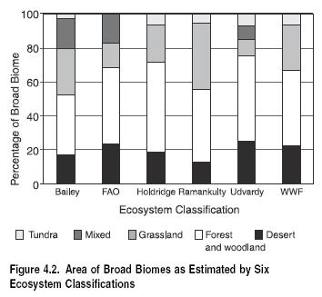
Different classifications serve different purposes and may yield different results. For example, the result of an analysis between five broad global [[biome]s] and six global terrestrial ecosystem classifications is shown in Figure 4.2. The ecosystem classifications were chosen to capture a range of the varying techniques that have been used to map ecosystem boundaries. The five broad biomes include desert (both hot and cold deserts), forest and woodland, grassland (includes grassland, savanna, steppe, and shrub), mixed, and tundra. The mixed class comprises the mixed mountain classes of FAO, the mixed mountain and island systems of Udvardy (1975), and the Mediterranean forests (Forest biome), woodland, and scrub class of WWF. It is difficult to divide mixed classes accurately between the remaining broad biome classes, so they were classified as a separate class.

There is reasonable agreement in area between some of the biomes and less agreement among others. The biomes that are reasonably consistent across ecosystem maps are forest and woodland, desert, and tundra. Delineation of grasslands is less consistent, and the reported grassland area differs across ecosystem maps by as much as 30%. Forest and woodland, the most predominant biome, is represented at between 42% and 53% of the terrestrial land surface (approximately 55 million to 73 million square kilometers). These results illustrate the implications of different choices of global ecosystem classifications for assessment, particularly as relates to the grassland biome.

Table 4.2 illustrates the methods used to define the ecosystem boundaries, the purpose for which they were classified, and the scale at which they were mapped. These are variables that should be considered in order to determine the appropriateness of a classification for a particular assessment.

In this chapter and elsewhere in this assessment, the WWF terrestrial biomes, built up from the classification of terrestrial ecoregions, were chosen to assess magnitude, distribution, condition, and trend of terrestrial biodiversity. (See Figure 4.3 in Appendix A.) Currently there is no equivalent classification for [[marine] ecosystems]. A separate set of freshwater (Freshwater biomes) biomes, used to classify freshwater ecoregions, is in preparation by WWF and The Nature Conservancy.

4.2 Current Status of Biodiversity

This section presents information on the global status of biodiversity, measured at the scale of biogeographic realms, biomes, species, populations, and genes. Under each heading, the significance of that level is introduced, followed by information on what is known about its current condition

4.2.1 Biogeographic Realms

Biogeographic realms are large spatial regions within which ecosystems share a broadly similar biota. Eight terrestrial biogeographic realms are typically recognized, corresponding roughly to continents (for example, the Afrotropical realm). Terrestrial biogeographic realms reflect freshwater biodiversity patterns reasonably well, but marine biogeographic realms are poorly defined.

4.2.1.1 Definition and Measurement

Similar ecosystems (tropical moist forests, for instance) share processes and major vegetation (Land-cover) types worldwide, but their species composition varies markedly among the world’s eight biogeographic realms (Olson et al. 2001). For example, the major tree species in tropical moist forests in Southeast Asia differ from those dominating tropical moist forests in South America. There is substantial variation in the extent of change and degradation to biodiversity among the biogeographic realms, and they face different combinations of drivers of change. In addition, the options for mitigating or managing drivers vary among realms. Although realms map roughly onto continents, they differ from continents in important ways as a result of biogeographic history.

4.2.1.2 Current Status of Biogeograpical Realms

Biogeographic realms vary widely in size. The largest is the Palearctic, followed by the Afrotropical and Nearctic realms; the smallest is Oceania. (See Table 4.3.) These area estimates are based on terrestrial area only, although the realm boundaries can be applied to inland water ecosystems with slight modifications of the boundaries to ensure that they do not cut across freshwater ecoregions or [[biome]s] (habitat types). Among terrestrial realms, net primary productivity (Imhoff et al. 2004) and biomass (Olson et al. 1980) values are highest in the Neotropics, followed closely by the Afrotropical and Indo-Malayan realms. The least productive is the Antarctic realm.

Land cover composition also varies widely between realms. Because realms are defined biogeographically, and not by dominant habitat type, each realm typically contains a mix of land cover types as mapped by GLC2000 (USGS-EDC 2003). (See Figure 4.4 in Appendix A.) Some biogeographic realms, however, are dominated by a single land cover type. For example, more than 40% of the Australasian realm consists of herbaceous cover and more than 40% of the Neotropics consist of broadleaf forests. In each biogeographic realm, significant areas have been converted from native habitats to agriculture and urban land uses. All realms have experienced at least 10% habitat conversion, and the Indo-Malayan realm has by far the largest percentage of agricultural and urban lands (54%).

Partly in response to this land conversion, nations in all biogegraphic realms have designated formal protected areas to conserve native ecosystems. Protection (IUCN classes I–IV) (WCMC 2003) of terrestrial biogeographic realms ranges between 4.0 and 9.5%. The realms with the greatest proportion of protected land area are Oceania (9.5%) and the Nearctic (7.8%). The Indo- Malayan (4.8%) and Palearctic (4.0%) realms contain the lowest proportion of protected land area. The Palearctic is the largest, and although only 4.0% is protected, it contains the largest total protected land area. The vast majority of protected areas have been designed to protect terrestrial ecosystems and biodiversity features, which has led to relative under-protection of inland water and marine biodiversity. (See Chapters 18, 19, and 20.)

The extent of inland water systems is greatest in the Nearctic and Palearctic realms (for example, lakes and peatlands). The Nearctic realm has by far the largest proportion of the world’s lakes (Revenga and Kura 2003). In terms of water volume, however, the Neotropic and the Indo-Malayan realms contribute the most discharge into the oceans. Australasia contributes the least, with only 2% of the world’s freshwater discharge (Fekete et al. 1999). The extent and distribution of inland water ecosystems has not been exhaustively documented at the global or regional scale. And while the biogeographic and ecological classification of inland water ecosystems is less well developed than for terrestrial ecosystems, more than 50 classifications are in use (see, e.g., Asian wetland classification system: Finlayson 2002; Darwall and Revenga in prep).

Each biogeographic realm contains a range of major habitat types or biomes. The Indo-Malayan, Oceanic, and Neotropical realms are dominated by tropical forest and [[grassland] biomes], while the polar realms (Palearctic, Nearctic) contain higher proportions of tundra and boreal forest. The Afrotropics are dominated by tropical grasslands. Although dominated by different biomes, most realms contain similar biome richness. All but Oceania include 9–11 of the 14 terrestrial biomes. Oceania is composed mostly of low, tropical islands and is dominated by tropical forest and tropical grassland biomes.

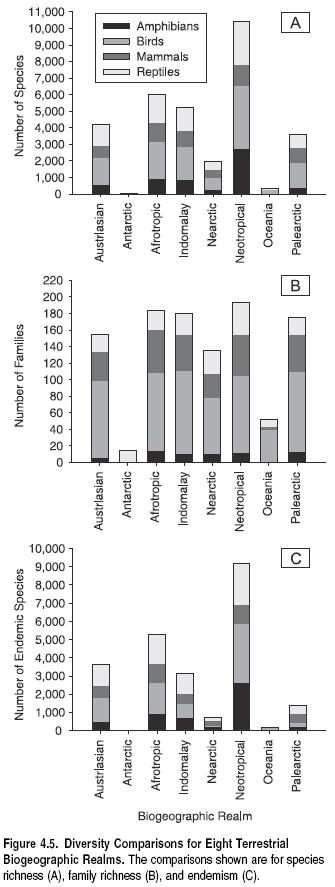
In part due to differences in biome richness and composition, biogeographic realms differ markedly in species and family richness, at least for the four vertebrate classes for which data exist. Figure 4.5 shows species richness among realms based on presence or absence records of terrestrial vertebrates (birds, mammals, and reptiles) in each of the 825 WWF terrestrial ecoregions (WWF 2004). This is supplemented by an analysis of extent of occurrence polygon data for amphibians and threatened birds (Baillie et al. 2004; BirdLife 2004b). The Neotropics are by far the most species-rich realm, both overall for terrestrial vertebrates and for each of the four taxa. (See Figure 4.5a.) Other realms containing high proportions of tropical forests (such as Indo-Malayan) also show high species richness in terrestrial vertebrates. With the exception of Antarctica, Oceania is the least species-rich realm due to its small overall land area and the relatively species-poor faunas typical of islands.

Biodiversity at the level of families is more similar among biogeographic realms (see Figure 4.5b) except for Oceania and Antarctica. These patterns differ somewhat among some inland water groups. The Neotropics have more than twice as many freshwater fish families as the Nearctic and Palearctic, and the Afrotropic and Indo-Malayan realms are only slightly behind the Neotropics (Berra 2001).

The number of species restricted to single realms (realm endemics) closely mirrors species richness patterns, at least for the four vertebrate classes assessed here. (See Figure 4.5c.) The Neotropics contain not only the greatest number of terrestrial vertebrate species but also the greatest number that occur only there. In all realms, however, the percentage of endemic species compared with total species richness is substantial (34–88%). Oceans, deserts, and other barriers to dispersal have resulted in vertebrate terrestrial faunas that are largely unique to each continent. We do not know how this pattern compares to patterns of realm endemism in nonvertebrates.

4.2.2 Biomes

4.2.2.1 Definition and Measurement

Biomes represent broad habitat and vegetation types and span across biogeographic realms (for example, the [[tundra] biome] is found in both Palearctic and Nearctic realms). Biomes are useful units for assessing global biodiversity and ecosystem services because they stratify the globe into ecologically meaningful and contrasting classes.

Throughout this chapter, and elsewhere in the MA, the 14 biomes of the WWF [[terrestrial] biome] classification are used, based on WWF terrestrial ecoregions (Olson et al. 2001). The nested structure of this classification, with finer-scale ecoregions nested into both biomes and biogeographic realms, allows assessments to be scaled up or down depending on the objectives. Furthermore, several datasets are already available and others continue to be associated with the WWF classification (such as vertebrate and plant species distribution data, threatened species, area-based estimates of net primary productivity, and land cover). The biome-level boundaries have very good resolution and accuracy, as they are based on the finer-scale ecoregions and are of an appropriate scale and number for global reporting.

These boundaries are based on the original or potential extent of these ecosystems or biomes, and do not take human-induced land cover changes into account. The extent of the ecosystems or biomes before the extensive changes brought about with the rise of the human population (Population growth rate) and industrialization in the modern era will probably never be known. We refer to this earlier, less altered state as ‘‘original,’’ while recognizing that climatic and environmental changes have always caused change and movements in Earth’s ecosystems. Therefore the global classifications can only be an approximation of the original boundaries of these ecosystems. The difference between original and current extent can be significant and forms an important component of the assessment of biodiversity loss.

There is no comparable global classification of freshwater (Freshwater biomes) biomes, but WWF and The Nature Conservancy are developing a major new biome classification for fresh water, to be completed in 2005. Terrestrial biomes tell us little by themselves about the size or type of freshwater habitat, which in turn has an enormous influence on the kind and number of species occurring there. For instance, a major river system can be adjacent to a very small basin, and both may fall within the same terrestrial biome, but they can contain vastly different assemblages of aquatic species. Freshwater biomes in the forthcoming classifications will be based largely on a combination of system size and type (such as large rivers versus small lakes), connectivity to coastal zones (such as total connectivity for islands), and overarching climatic conditions (such as temperate versus tropical or dry versus moist).

Like freshwater biomes, [[marine] biome] classification is less developed than that for terrestrial systems. The dynamic nature and the relative lack of natural boundaries in oceanic ecosystems make biogeographic divisions problematic, and there is no standard classification scheme. Nonetheless, several classifications of the marine realm exist, some based on biogeography (such as Briggs 1974), others on oceanographic and hydrological properties, and still others on ecological features, such as using the distribution of species assemblages in relation to seasonal characteristics of local and regional water masses (Ford 1999). Longhurst (1995) classified the world’s oceans into four ecological domains and 56 biogeochemical provinces, largely on the basis of estimates of primary production rates and their changes over time. (See chapter 18.) Hayden et al. (1984) subdivided Dietrich’s (1963) 12 marine realms into oceanic realms and coastal regions on the basis of physical and chemical properties including salinity, temperature, and seasonal movement of water and air masses.

Two marine classification systems have been used more widely. First, Bailey (also based on Dietrich 1963, 1998) includes oceanic ecoregions in his global classifications, mapping 14 marine divisions spread between the three domains. Continental shelves (less than 200 meters water depth) are distinguished; other divisions are delineated on the ocean surface based on four main factors: latitude and major wind systems (determining thermal zones) and precipitation and evaporation (determining salinity).

Second, Sherman and Alexander’s (1986) system of large marine ecosystems delineates 62 regions of ocean encompassing near-coastal areas from river estuaries to the seaward boundary of continental shelves and the seaward margins of coastal current systems. They are relatively large regions (greater than 200,000 square kilometers), characterized by distinct bathymetry, hydrography, biological productivity, and trophically dependent populations. This approach aims to facilitate regional ecosystem research, monitoring (Environmental monitoring and assessment), and management of marine resources and focuses on the products of marine ecosystems (such as the fish harvest). In general, no marine biome classification scheme has successfully covered the wide range of oceanic depths and addressed the lack of regional uniformity, thus complicating a global assessment of marine biodiversity.

4.2.2.2 Current Status of Major Terrestrial Biomes

The world’s 14 [[terrestrial] biomes] vary in total area by two orders of magnitude, from nearly 35 million square kilometers (deserts and dry shrublands) to 350,000 square kilometers (mangroves). (See Table 4.4.)

Biomes also vary widely in per-area measures of plant biomass (Olson et al. 1980) and net primary productivity (Imhoff et al. 2004). Net primary productivity is the net amount of carbon fixed by plants through photosynthesis (after subtracting respiration) and represents the primary energy source for the world’s ecosystems (Vitousek et al. 1986). Tropical moist forests show high levels of both standing biomass and annual productivity, while other biomes, such as temperate coniferous forests and boreal forests (Forest biome), have high biomass despite low annual (and more seasonal) productivity.

Each biome mapped in Figure 4.3, while typically dominated by the expected [[vegetation (Land-cover)] cover], actually comprises a complex mosaic of different land cover types as mapped by GLC2000. (See Figure 4.6 in Appendix A.) This heterogeneity is due in part to fine-scale mixture of ecosystems within these broadly defined biomes. For example, boreal forests are composed primarily of coniferous forest land cover but contain a substantial proportion of shrublands (Grassland biome) and [[grassland]s].

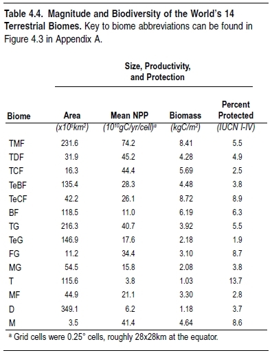
Another cause of land cover heterogeneity within biomes is conversion of native [[habitat]s] to agriculture, pastures, and other human land uses. Indeed, in over half the biomes, 20–50% of land area has been converted to human use. Tropical dry forests are the most affected by cultivation, with almost half of the biome’s native habitats replaced by cultivated lands. Three additional biomes— temperate grasslands, temperate broadleaf forests, and Mediterranean forests (Forest biome)—have experienced 35% or more conversion. Biomes least affected by cultivation include deserts, boreal forests, and tundra. While cultivated lands provide many provisioning services (such as grains, fruits, and meat), habitat conversion to intensive agriculture leads to reductions in native biodiversity.

Biomes differ widely in the percentage of the total area under protection. Table 4.4 shows the total area under protection, including only lands classified in the four highest IUCN Protected Area categories (IUCN 1994). Flooded grasslands, tundra, temperate coniferous forests, mangroves, and boreal forests have the highest percentage area under protection—perhaps because these biomes are among the least useful for competing land uses, such as agriculture. Conversely, temperate grasslands, Mediterranean forests, and tropical coniferous forests are the least protected biomes.

To compare species richness among biomes, a similar methodology used to determine species richness at the level of realms has been applied. Tropical biomes have the highest levels of overall species richness, as well as the highest richness for each of the four taxa analyzed. (See Figure 4.7.) This is true of tropical moist forest, but also, perhaps surprisingly, of tropical grasslands and savannas (Grassland biome) and tropical dry forests, the second and fourth richest biomes overall. Deserts and Mediterranean grasslands are also relatively rich biomes for terrestrial vertebrate species.

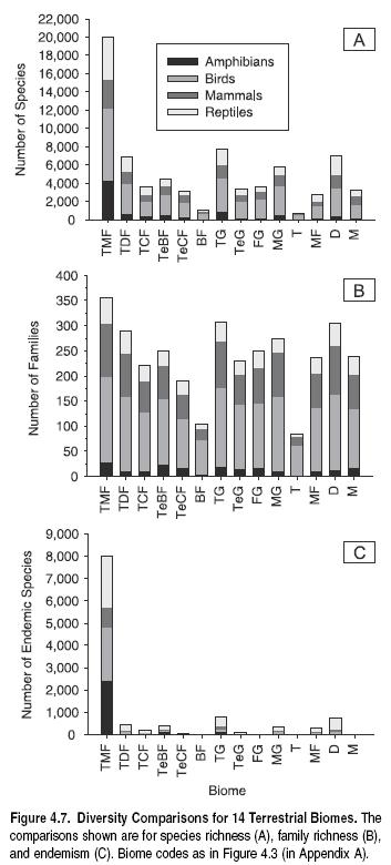
Tropical moist forests also contain the greatest diversity of higher taxa and therefore represent the greatest store of Earth’s evolutionary history. The five biomes richest in terrestrial vertebrate species are also the five richest in families, although differences among biomes are not as pronounced. Tropical moist forests, therefore, contain many more species per family on average, suggesting that this biome has experienced higher rates of species diversification within families.

The number of biome-endemic species—that is, species found in a certain biome and nowhere else—varies widely among biomes. Tropical moist forests contain by far the highest number of endemic species, an order of magnitude more than any other biome. This pattern again may be the result of high speciation rates in this biome, as well as relatively smaller range sizes in lower latitudes (Rosenzweig 1995; Gaston 2000).

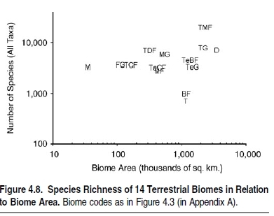
The relative richness of the world’s biomes, however, may be influenced by their relative sizes as well. Biomes vary enormously in area, as noted earlier, and species richness is well known to increase with the area sampled (Rosenzweig 1995). Therefore, although both tropical moist forests and tropical grasslands contain high total richness, this may be due in part to the fact that they represent two of the largest [[biome]s]. Figure 4.8 plots species richness against area for the 14 biomes. In fact, the two are not statistically related (p _ 0.75).

4.2.3 Species

The classification of living organisms into manageable groups greatly facilitates their study. The hierarchical system of classification used today is largely based on evolutionary relationships. The major categories, from the most inclusive to the smallest groups Kingdom-Phylum-Class-Order-Family-Genus-Species. It is at the level of species that living organisms are most widely known, both by common and scientific names.

4.2.3.1 Definition and Measurement

Although natural historians have been classifying living organisms into species since at least classical times, there is still no consensus on how this is best done (Hey 2001). Since the middle of the twentieth century, the dominant idea of how to define the term ‘‘species’’ has been the biological species concept (Mayr 1963), which defines species as groups of interbreeding natural populations whose members are unable to successfully reproduce with members of other such groups. Gene flow within a species leads to cohesion, whereas the lack of gene flow between different species means they are independent evolutionary lineages. Species therefore have natural and objective boundaries under this view, and so are natural units for biodiversity assessment.

Another hierarchy to which species belong is the evolutionary ‘‘family tree,’’ or phylogeny, that links them all. In some well-studied groups (such as angiosperms (APG 1998) and birds (Sibley and Monroe 1990)), current taxonomic classification largely (and increasingly) reflects evolutionary relationships, such that species in a given taxon are all thought to share a more recent common ancestor with each other than with species in other taxa. Higher taxonomic groupings then represent increasing levels of independent evolutionary history. In less well known groups, by contrast, classifications may not (and may not even attempt to) reflect phylogeny.

Regardless of how phylogenetic groups are recognized and named, decisions about the taxonomic rank (genus, family, and so on) of the various groups are arbitrary (Avise and Johns 1999). Many genera of insects, for instance, originated earlier than most avian families. Unlike biological species, higher taxonomic categories and lower taxonomic categories, like subspecies or races, have no natural boundaries.

Therefore species have advantages over other levels in the classificatory hierarchy and are useful units for biodiversity assessment. Some problems with using species as a unit for biodiversity assessment remain—both theoretical and practical; they can often be overcome or ameliorated with care, but they should never be overlooked (Isaac et al. 2004; Mace 2004). (See Box 4.1.)

BOX 4.1 Species in Theory and Practice

Species concepts based on gene flow and its limits, such as the biological species concept, are not applicable to asexual taxa. They are also inadequate for ‘‘pansexual’’ taxa, such as some bacteria, where gene flow can be common between even very dissimilar types. However serious these concerns are in theory, they rarely matter for biodiversity assessment because the data collected on such groups are usually insufficient for problems to emerge. These and other issues have, however, led to a proliferation of species concepts: there are dozens in current use (Claridge et al. 1997; Mayden 1997), though most share the feature that species are independent evolutionary lineages. Most of the concepts—whether based on gene flow, ecological separation, or morphological distinctiveness—tend to give similar answers in most cases, for two reasons. First, most species have a considerable history of independent evolution—maybe millions of years—and have evolved morphological, ecological, and reproductive characters that set them apart from other species. Second, most populations within species share common ancestors with other populations in the very recent past, so they are barely differentiated at all. Borderline cases, where different criteria disagree, are relatively rare (Turner 1999). Application of the phylogenetic species concept, however, may lead to the recognition of very many more species than when other concepts are used. A phylogenetic species is ‘‘the smallest group of organisms that is diagnosably distinct from other such clusters and within which there is a parental pattern of ancestry and descent’’ (Cracraft 1983); any diagnosable difference, however small, is deemed a sufficient basis for describing a new species. Taxonomic revisions that apply this concept to a taxon for the first time typically roughly double the number of species recognized (Agapow et al. 2004). Most theoretical species concepts, like the biological one, are not very operational: they define the sort of entity a species should be but do not provide a method for delimiting them (Mayden 1997). In practice, simpler, perhaps informal decision rules are typically used to determine how many species to describe (Quicke 1993), with these rules differing among major taxa (Claridge et al. 1997). Even within a group, taxonomists lie on a continuum from ‘‘lumpers’’ (who recognize few species, which will consequently tend to be widespread) to ‘‘splitters’’ (who recognize many species, which often have restricted distributions), with obvious consequences for biodiversity assessment (Hull 1997). The recognition that a full catalogue of the world’s species is hundreds of years away, at current rates of description, has prompted initiatives to simplify the jobs of describing and defining animal and plant species (Godfray et al. 1999; Hebert et al. 2003; Tautz et al. 2003) and calls for a program to sequence DNA from all the world’s biota (Wilson 2003). These initiatives are controversial and are currently only at the trial stage. Species are the major taxonomic unit for counting biodiversity: species lists are important for both monitoring (Environmental monitoring and assessment) and broad-scale priority setting (Mace et al. 2003). However, species may differ in the weighting they receive, to reflect differences in their perceived biodiversity value. In addition to species of recognized economic importance, four other categories of species that might receive more weight are keystones (whose loss from a system would lead to large-scale changes in it), indicators (Indicator species) (whose sensitive requirements mean that their abundance reflects overall system health), flagships (charismatic species whose plight attracts publicity), and umbrellas (flagships whose conservation in situ would automatically help conserve many other species) (Meffe and Carroll 1994). More weight might also be assigned to species that are at risk of extinction, or rare, or the have restricted distributions (e.g., Myers et al. 2000). There is no consensus about exactly how any of these weights should be determined nor their relative importance. Phylogenetic information can also be considered, by weighting species or locations according to the amount of unique evolutionary history they embody (Vane-Wright et al. 1991; Faith 1992). These ways of augmenting information in species lists may be of little use when species lists are very incomplete (Mace et al. 2003), which they can be for even well-known taxa. Then, any comparisons between regions, systems, or taxa that do not control for variation in sampling effort run the risk of serious error. The picture is even cloudier when sampling effort differences are compounded with differences in species concept. Counts of higher taxa (such as genera or families) might be more robust than species counts to sampling differences among regions, and so they may be pragmatic choices despite the loss of precision incurred (Balmford et al. 1996). Some very broad-scale comparisons among groups (bacteria versus mammals, for example) are practically meaningless because the differences in taxonomic practice are so great (Minelli 1993). Comparisons over time are hampered by the taxonomic instability that results from discovery of new species and changes in species concepts and by changing information about previously known species (Mace et al. 2003). Because of these considerations, the interpretation of biodiversity measures based on species numbers is not always straightforward. Such measures are most likely to be useful when the taxonomy of the group is apparently almost complete (that is, few species remain to be discovered), when the sampling and taxonomic effort has been equal among the units being compared, or when sampling and effort have at least been measured in a way permitting correction for sampling biases. In addition, it is clearly important that taxonomic practice, including the choice of species concept, be reasonably consistent. These requirements mean that species-based approaches are much more useful when applied to unusually well known taxa or well-known parts of the world (such as birds and mammals or Northern temperate regions) rather than to other taxonomic groups or less well documented systems (such as nematodes or freshwater (Freshwater biomes) and marine systems). The wealth of data available for the best-known groups permits very useful comparisons to be made between places in, for example, how many species there are, how many are threatened with extinction, or how many are threatened by overexploitation. However, patterns seen in a single group may be specific to that group (Prendergast et al. 1993). Different lineages have different ecological requirements and biogeographical histories, so they naturally may have different patterns of diversity and trends: consequently, no single taxon is sure to be a good surrogate for biodiversity as a whole. If comparisons are intended to reflect overall biodiversity, they should therefore be replicated using multiple taxa wherever possible.

4.2.3.2 How Many Species Are There?

Estimates of the total number of eukaryotic species vary greatly, most commonly falling between 5 million and 30 million (May 1992). The uncertainty stems from the fact that most taxonomic work is concentrated away from the most species-rich taxa (Gaston and May 1992) and regions (Gaston 1994a). In addition, the intensity of taxonomic work is actually declining (Godfray 2002). The discussion here is restricted to eukaryotic species. In the prokaryotes, different methods for recognizing and naming species, as well as severe problems with incomplete knowledge, make assessments and comparisons of species richness unreliable (Ward 2002; Curtis et al. 2002; Nee 2003).

Many methods of estimating total species numbers are based in some way on numbers of known, named species. Uncertainties around these estimates themselves pull in opposing directions. On the one hand, the lack of comprehensive systematic databases results in underestimates of known species numbers (Sugden and Pennisi 2000). On the other hand, the extent of synonomy between named taxa results in overestimates (May and Nee 1995). Several ongoing initiatives, such as Species 2000, the Integrated Taxonomic Information System, and the Global Biodiversity Information Facility, aim to eliminate these problems by providing up-to-date, electronic catalogues of known species (Bisby et al. 2002).

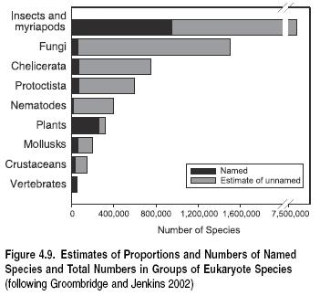
In total, summing across taxa suggests that the number of known species on the planet lies at around 1.75 million (Heywood and Watson 1995; Groombridge and Jenkins 2002). (See Figure 4.9.) It has, however been shown that some of these figures are underestimates; for example, mollusks are now believed to number 100,000 known species (Peeters and Van Goethem 2003). Further, current rates of species description average 15,000 species per year (Stork 1993), less than 1% of the known total, and hence at least another 135,000 species are likely to have been described over the decade since 1995, bringing the total of known species toward 2 million (Peeters et al. 2003).

A range of techniques exist for estimating the total species richness of the planet (May 1988). These can be grouped into two main classes (Stork 1997)—methods based on ratios of known to unknown species and those based on the extrapolation of samples (see Table 4.5)—with more speculative techniques based on scaling rules between species and body size (May 1990a), specialist opinion (Gaston 1991), and community pattern (Godfray et al. 1999).

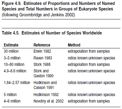
Methods based on ratios between known and unknown species have a long history but were first brought to high profile by Raven (1983). Specifically, he extrapolated the known 2:1 ratio of tropical to temperate vertebrate species to the existing 2 million known species—most of which are temperate insects—to estimate that there should be two as-yet-undescribed tropical insects for each temperate species, for a total of 3–5 million species. Stork and Gaston (1990) used similar logic (based on the percentage of British insects that are butterflies) to estimate the total numbers of insects at 4.9–6.6 million. Hodkinson and Casson (1991) extrapolated the percentage of undescribed Hemiptera in samples from Sulawesi to all insects, suggesting a total of 1.84–2.57 million species, while Hodkinson (1992) generalized this argument to suggest the number of species could be estimated at approximately 5 million, based on percentages of undescribed species in studies from the tropics.

The development of the second method—extrapolation of samples—is much more recent and was first developed by Erwin (1982). In studies of beetle species inhabiting tropical trees on Panama, he recorded high levels of both richness and local endemism. Extrapolating these figures globally, he estimated the total number of species at 30 million. His assumptions and methods have been tested and refined (Stork 1988; Hammond 1994; Ødegaard 2000; Sørensen 2003; Novotny et al 2002), and this method now suggests a lower global species richness of 4–6 million.

In general, there continues to be much debate in the literature regarding estimates of species richness, even among well-studied groups such as the extant seed plants. Lower estimates for seed plants range from 223,000 (Scotland and Wortley 2003) to 270,000 and 320,000 (May 1992; Prance et al. 2000), while higher estimates range up to 422,000 (Govaerts 2001; Bramwell 2002), although the higher figure is somewhat controversial (Thorne 2002; Scotland and Wortley 2003).

Several other particularly poorly known groups of organisms present additional problems for the estimation of global species richness (May 1995). Based on extrapolations of box-core samples from the seafloor, Grassle and Maciolek (1992) suggested a total of 10 million marine macrofaunal species; this may be rather high, but clearly enormous deep-sea species richness remains undiscovered. Likewise, the known global total of 72,000 fungi is certainly a large underestimate; based on the ratio of fungi to plants in Britain, Hawksworth (1991) estimated the global number to be closer to 1.5 million. Maybe most important, parasitic richness remains largely unknown: if the possibility that there is at least one host-specific parasite for all metazoan or vascular plant species is borne out (Toft 1986), the number of estimated species could double.

4.2.3.3 Variation in Species Richness in Time and Space

While the number of species on the planet is hard to estimate, its variability across space and time is much harder. Nearly all patterns of species richness are known with greater confidence for terrestrial than for either marine or freshwater (Freshwater biomes) systems. Species are unevenly distributed over Earth’s surface (Rosenzweig 1995) and across phylogenetic space: species’ ages and histories vary widely (May 1990b). Considerable data have recently been compiled that allow the identification of numerous patterns of variation, but these remain restricted to tiny subsets of all species, and so their general applicability remains unknown. Nevertheless, for lack of any truly comprehensive datasets, these data form the basis for the rest of this section.

For many purposes, species are not all equal—in particular those species with long independent evolutionary histories and few surviving relatives contain irreplaceable genetic diversity. Measures of phylogenetic diversity reflect this and can sometimes be approximated by higher taxon diversity.

Global species richness maps exist for mammals (terrestrial species only) (see Figure 4.10 in Appendix A), amphibians (see Figure 4.11 in Appendix A), sceleractinian corals (Veron 2000), the 239 bumblebee species of the genus Bombus (Williams 1998), marine finfish species across FAO region and freshwater finfish by continent (Froese and Pauly 2003) (see Figure 4.12 in Appendix A), plants (see Figure 4.13 in Appendix A) (Barthlott et al. 1999), and freshwater fish by river basin (multimedia.wri.org/water sheds_2003/gm2.html). The lack of distributional data for invertebrates generally (in particular, for aquatic species) is clearly a major limitation on inference from these data; some regional data sets exist, but these are so heavily skewed toward north temperate regions as to have limited value in a global assessment. Another limitation of these data is their static nature: they reflect current extent of occurrence, not historical range, which can often be very different (Channell and Lomolino 2000), and they fail to reflect temporal variation within species’ ranges—for example, for migratory species (Go´mez de Silva Garza 1996). Further limitations come from wholesale sampling artifacts: for instance, the Congo Basin and New Guinea are particularly poorly sampled for all taxa, likely leading to an underrepresentation of species richness in these areas.

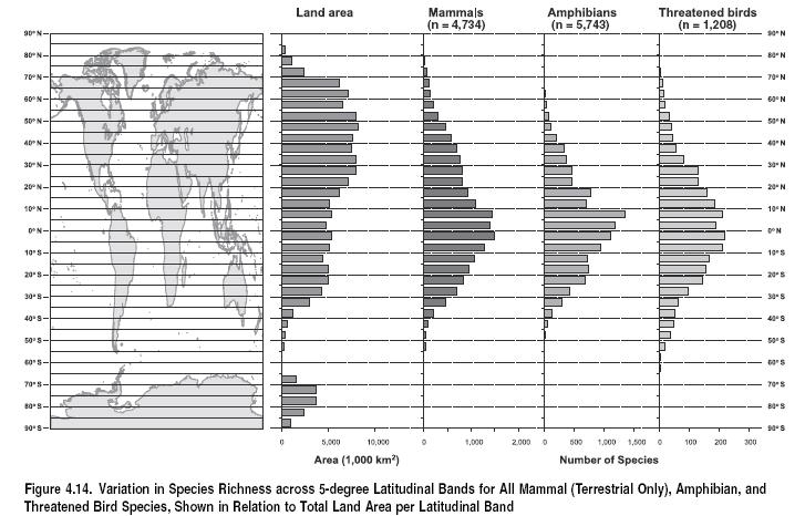
The most obvious pattern emerging from these data is that for most taxa the tropics hold much higher species richness than do the temperate, boreal, and polar regions. Figure 4.14 demonstrates this by plotting the number of species in each 5-degree latitudinal band for all terrestrial mammals, threatened birds (as global bird data are not yet available), and amphibians. As expected from the species-area relationship (Rosenzweig 1995), some of this pattern is explained by variation in landmass across latitudinal bands. However, species richness is much higher in the tropics than would be expected based on area alone, peaking around the equator for all taxa (rather than in northern high latitudes, as would be predicted based on area alone).

The other pattern apparent from Figures 4.10–4.13 is the broadly similar distribution of diversity between taxa. Thus, for example, species richness per grid cell is tightly correlated between mammals and amphibians. Differences seem likely to be driven by particular biological traits. Birds, for example, have the ability to disperse over water more than most of the taxa mapped here, and so occur in larger numbers on islands, while ectothermic reptiles flourish in desert regions generally impoverished in other taxa. Other differences are less easily explained, such as the high richness of mammal species in East Africa and of amphibians in the Atlantic forest. In general, these differences will increase with increasing evolutionary distance (and hence often corresponding ecological differences) between taxa (Reid 1998): less correlation is expected between mammal and coral distributions, for instance, than between mammal and bird distributions.

Macroecological patterns of freshwater and marine species richness are less well understood. Diversity of pelagic predators seems to peak at intermediate latitudes (20–30^o N and S), where tropical and temperate species ranges overlap (Worm et al. 2003). Several studies have documented a latitudinal gradient in the shallow-water benthos, with decreasing richness toward the poles, but data on nematodes suggest that no latitudinal trend exists (see Snelgrove 1999, and references therein). A recent global assessment of local stream insect richness found peaks in generic richness near 30–40^o N latitude, though the study compared individual stream surveys rather than summing values across all latitudinal bands (Vinson and Hawkins 2003).

4.2.3.4 Geographic Centers of Endemism and Evolutionary Distinctiveness

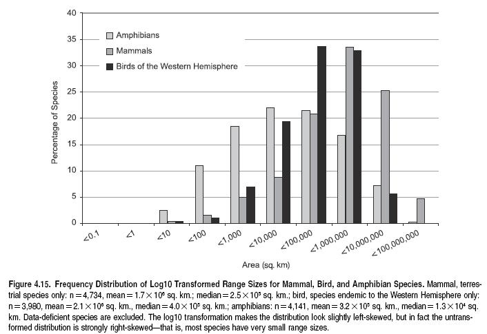
Interacting with geographic variation in species richness is variation among species in range size. Most species have small range sizes (Gaston 1996), although there is variation within this general pattern. Among the vertebrates, the more mobile species, such as birds, tend to have large ranges, while those of less mobile species, such as amphibians, generally have much smaller ranges. (See Figure 4.15.) Nevertheless, the shape of frequency distributions of species’ range sizes appears to be similar across all taxa examined to date (with the median range size consistently an order of magnitude smaller than the mean), probably because shared processes are shaping these distributions (Gaston 1998). The small range size of most species has important consequences for the conservation of biological diversity, given the widespread inverse correlation between species’ range size and extinction risk (Purvis et al. 2000b).

Not only do most species have small ranges, but these narrowly distributed species tend to co-occur in ‘‘centers of endemism’’ (Anderson 1994). Such centers have traditionally been identified through the overlap of restricted-range species, found using threshold approaches that consider only species with distributions smaller than a given percentile or area (Hall and Moreau 1962). Among vertebrates, almost all such centers of endemism lie in isolated or topographically varied regions. This is true for both [[geographic]al] isolates, such as mountains and peninsulas, and real land isolates—islands (Baillie et al. 2004). Maybe as a consequence of this, they also tend to be near the coast.

The degree to which this pattern is found for other taxa, and in particular in the aquatic realm, is unclear, but evidence from analysis of scleractinian corals and selected fish, mollusks, and lobsters suggests that coral reef centers of endemism also tend to be isolated, either by distance or by current flow (Roberts et al. 2002).

Centers of endemism are also concentrated in the tropics. Centers of endemism across birds, mammals, and amphibians tend to overlap (Baillie et al. 2004), and a broadly similar pattern is expected for plant endemism as well (WWF and IUCN 1994, 1995, 1997; Myers et al. 2000), although Mediterranean regions are more important as centers of endemism for plants than for vertebrates.

The range area and endemism patterns characteristic of the vertebrates (as well as of the plants, possibly) do not appear to represent the situation for invertebrates or microorganisms. Despite the fact that the data are extremely sparse and species have rarely been comprehensively identified locally, let alone mapped, various lines of evidence suggest that patterns of spatial turnover for these groups may be very different. While it is known that local endemism can be very high for some invertebrates in certain areas, this measure—calculated as the ratio of local to regional richness—varies widely. In Amazonia, for example, these ratios varied from about 80% for some moth species (indicating low endemism) to less than a few percent for earthworms (indicating very high endemism and spatial turnover) (Lavelle and Lapied 2003).

Species richness in soils is important for many ecosystem processes, but this habitat has been relatively poorly studied compared with aboveground systems (Fitter 2005). Microbial diversity is known to be high, though quantification at both local and global scales is limited by the technical issues of standardizing methods for defining microbial species. Richness of larger soil organism varies: some groups appear to be locally very diverse relative to global or regional diversity. This seems to be especially the case for smaller organisms and those with high dispersal abilities (through wind and water, for instance). Currently poorly understood, species richness in soils may be best explained through a better understanding of the temporal and spatial variability of the physical properties of soil as a habitat (Fitter 2005).

More generally, it has been suggested that the extent of local endemism correlates negatively with the dispersal capabilities of the taxon. Interpreting this pattern more broadly, and using extensive inventories of free-living protists and other microbial eukaryotes in a freshwater pond and a shallow marine bay, Finlay and Fenchel (2004) suggested that most organisms smaller than 1 millimeter occur worldwide wherever their required habitats are found. This can result from almost unrestricted dispersal driven by huge population sizes and very small body size, with the consequently low probability of local extinction. Organisms larger than 10 millimeters are much less abundant and rarely cosmopolitan. In Finlay and Fenchel’s data, the 1–10 millimeter size range accommodates a transition from a more-or-less cosmopolitan to a regionally restricted distribution.

More detailed studies can reveal different spatial richness patterns within taxa and in different major [[biome]s]. For example, in one study of Neotropical mammals, dryland habitats were shown to be more diverse in endemic mammalian species than were the tropical forests (Mares 1992). Marine biota reveal a similar overall decline in diversity with increasing latitude to that observed in terrestrial realms, but the strength and slope of the gradient are subject to regional, habitat, and organismal features (Hillebrand 2004). Detailed studies of the species richness of fish and invertebrates in the Atlantic showed no clear trends but seemed to be related to sea-surface temperature or nitrate concentrations (Macpherson 2002).

In addition to the variability of species richness across geographic space, species richness varies over time. There is enormous variation between species in terms of their evolutionary age or the time since divergence from their closest relative (Faith 1992). Comprehensive phylogenetic data allowing evolutionary relationships to be drawn across entire species groups remain sparse. However, it is possible to use taxonomic relationships to approximate evolutionary relationships (Vane-Wright et al. 1991) in order to measure evolutionary distinctiveness among species. As with species richness, the few data that exist for terrestrial taxa indicate that tropical rainforests are regions with the greatest number of taxa with lengthy independent evolutionary history—for example, for plant families (Williams et al. 1994) and primates and carnivores (Sechrest et al. 2002). The applicability of this variation in higher taxon diversity in aquatic systems remains largely untested, however, and the massive phylum diversity in the sea (32 of 33 phyla occur in the sea, compared with just 12 on land) suggests some important differences here (May 1994).

Based on the notion that conserving global biodiversity requires preserving these spatial and temporal patterns, one recent analysis investigated the extent to which [[species (Species diversity)] diversity] is covered by the current network of protected areas (Rodrigues et al. 2004). The analyses were based on distribution maps of 11,633 species of terrestrial vertebrates and found that at least 12% of all species analyzed do not occur in protected areas. This rises to 20% of threatened species, the loss of which would result in the disappearance of at least 38 threatened genera. (See Table 4.6.) Most species not found in protected areas are concentrated in tropical regions, and within these in centers of endemism: mainly islands and tropical mountain areas (Rodrigues et al. 2004).

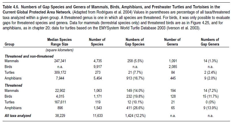
Equivalent analyses are not possible yet for hyper-rich taxa such as plants or insects. However, the results for vertebrates indicate that taxa with higher levels of endemism (smaller range sizes) are proportionally less covered by protected areas; if so, the number of plant and insect species not found in any protected areas may be higher than for terrestrial vertebrates (Rodrigues et al. 2004). Freshwater species are also likely to be poorly covered, as most currently existing protected areas were not created focusing on freshwater habitats; even when species-rich freshwater systems occur in protected areas, they are not necessarily protected. The coverage of marine richness is surely tiny, with only about 0.5% of the world’s oceans covered by protected areas (Chape et al. 2003).

4.2.4 Populations

4.2.4.1 Definition and Measurement

The term population is used in many different fields and at many scales, resulting in a number of different definitions (Wells and Richmond 1995). Most definitions identify a population as a geographical entity within a species that is distinguished either [[ecological]ly] or genetically (Hughes et al. 1997). The genetically based definition (‘‘Mendelian population’’) is a reproductive community of sexual and cross-fertilizing individuals that share a common gene pool (Dobzhansky 1950). This is measured by assessing gene flow and genetic variation. The demographically based definition identifies populations based on groups of individuals that are sufficiently isolated to have independent population dynamics (Luck et al. 2003).

For some purposes, it is useful to categorize groups of organisms that may not correspond to a Mendelian or demographic population. For example, a group of bees in a field might be a population worthy of study. A population can also be defined as a unit that is important for conservation (conservation unit), such as evolutionary significant units, (Moritz 1994; Crandall et al. 2000) or for management (management units), such as fish stocks. Populations may also be defined in relation to the services that they provide. Thus, a service-providing unit would be that section of a population that is essential for providing a specific ecosystem service (Luck et al. 2003).

The definition of population used in the MA is more general and could lead to a number of different interpretations of a population’s boundary. It is ‘‘a group of individuals of the same species, occupying a defined area and usually isolated to some degree from other similar groups.’’ Specification of the way in which the term population is being used is clearly important, given the great diversity of uses of the term.

4.2.4.2 Current Status of Population-Level Biodiversity

Populations are an important aspect of biodiversity as they are widely understandable units and are the ones most often monitored, exploited, and managed by people. Change in the status of populations provides insight into the status of genetic diversity, as the extinction of a population may represent the loss of unique genetic material. Populations are also the level at which we can best observe the relationship between biodiversity and ecosystem functioning. Most of the services provided by ecosystems require a large number of local populations (Hughes et al. 1997). For example, erosion control requires a number of different local plant populations. The loss of these local populations may have profound effects on erosion but limited impact on the overall status of the species involved. Thus it is important to focus on the condition of local populations if we are concerned with the maintenance of ecosystem processes and the provision of ecosystem services.

There are a number of ways that the condition of populations can be measured: the total number of populations in a given area, the total number of individuals within each population, the geographic distribution of populations, and the genetic diversity within a population or across populations (Luck et al. 2003). The most common measures are [[assessment]s] of the distribution and abundance.

Populations are dynamic and are continually changing due to variation in births and deaths, immigration, and emigration. At any one time a species will likely have some populations that are increasing while others are decreasing, and it may be going extinct. A species can have many different structures, ranging from one continuous population of individuals, to disjunct populations of individuals with some exchange of individuals among them (known as a metapopulation) (Wells and Richmond 1995) and to disjunct populations that are completely isolated. Although there is great variation in abundance and distribution, the majority of species have small distributions (see Hughes et al. 1997) and therefore small populations. Small numbers of individuals or limited distributions result in such populations being more susceptible to extinction due to stochastic events (Gilpin and Soule´ 1986; Lande 1993) such as a hurricane or fire, random demographic effects (Richter-Dyn and Goel 1972; Goodman 1987), the potential negative effects of limited genetic variability (Soule´ 1980); or simply because a threat process such as habitat loss, exploitation, or introduced species is more likely to drive to extinction a species that is restricted in distribution or composed of few individuals.

Given the magnitude of populations, it is little surprise that there are few comprehensive global datasets. One example is the global inventory of population estimates and trends for waterbirds maintained since 1996 by Wetlands International. The most recent (third) edition (Wetlands International 2002) listed 2,271 biogeographic populations of 868 species of waterbirds. Other organizations, such as IUCN–the World Conservation Union, BirdLife International, NatureServe, UNEP World Conservation Monitoring Centre, FAO, and the European Nature Information System, collect data on species distributions and in some cases populations.

But the quality of the population data remains poor, and where data do exist the species tend to be either commercially important (such as fish stocks), charismatic (such as tigers and elephants), or threatened with extinction. There is also a significant regional bias, with the least data available in regions such as the tropics, where population numbers are likely the highest. Another useful source of data for trends on populations is the Global Population Dynamics Database (NERC 1999), with 5,000 separate time series available, ranging from annual counts of mammals or birds at individual sampling sites to weekly counts of zooplankton and other marine fauna.

Despite these limitations, population-level information is extremely useful for a range of applications for assessments of biodiversity and ecosystem services.

4.2.5 Genes and Genomes

Genes are sequences of nucleotides in a particular segment (locus) of a DNA molecule. Slightly different sequences (alleles) at a locus may result in protein variants differing in amino acid sequence, which may have different biochemical properties and thus cause phenotypic differences in morphology, physiology or the behavior of individuals. The allele that causes sickle-cell anemia in humans, for example, is the result of a single nucleotide substitution (adenine replaced by guanine) in the second position of the sixth codon of the beta-globin gene.

The complete genetic material of a species constitutes its genome. Eukaryotic genomes are organized into discrete longitudinal bodies in the nucleus, called chromosomes. The number, size, and shape of chromosomes within species are usually constant, but often differ between species. The human genome has 46 chromosomes and about 3.2 billion nucleotides, containing about 30,000 to 40,000 genes.

Biodiversity at the within-species level is usually measured by genetic diversity, which refers to the variety of alleles and allele combinations (genotypes) present in a species. Genetic diversity is reflected in the differences among individuals for many characters, from DNA sequences and proteins to behavioral and morphological traits such as eye, skin, and hair color in humans. This diversity allows populations to evolve by means of changing relative frequency of different alleles to cope with environmental changes, including new diseases, pests, parasites, competitors and predators, pollution, and global change. Naturally outbreeding species with large populations usually possess large stores of genetic diversity that confer differences among individuals in their responses to any environmental change.

Numerous species have been observed to evolve in response to environmental change as a result of genetic diversity. For example, industrial melanism has evolved in about 200 species of moths in areas subject to industrial pollution (Majerus 1998), and resistance to insecticides, herbicides, antibiotics, and other biocontrol agents has evolved in numerous ‘‘pest’’ species (McKenzie 1996).

The plentiful genetic diversity in many plant and animal species has been exploited extensively by humans through artificial selection to generate numerous breeds specialized in providing various service products such as meat, milk, eggs, fiber, guidance, hunting, companion, and aesthetics. (See also Chapter 10 for a discussion of genetic bioprospecting.) In contrast, species lacking genetic diversity usually have difficulty adapting to environmental changes and face increased risk of extinction because any environmental change that harms one individual is likely to harm other individuals to a similar extent. It has been demonstrated that inbred populations lacking genetic diversity have lower fitness and are less adaptable to new environmental challenges than the outbred populations they are derived from (Reed et al. 2003).

Genetic diversity is also important in maintaining the reproductive and survival ability (reproductive fitness) of individuals in outbreeding species even in a stable environment. In naturally outbreeding species, loss of genetic diversity usually leads to the homogeneity within individuals and thus reduced reproductive fitness (inbreeding depression) and increased risk of extinction. The U.S. endangered Florida panther, a subspecies restricted to a small relic population of approximately 60–70 individuals in southern Florida, has very low levels of genetic diversity revealed by different genetic markers. As a result, Florida panthers suffer from inbreeding depression evidenced by an extraordinarily high frequency of morphological abnormalities (‘‘cow lick’’ patterns in their fur and kinked tails), cardiac defects, undescended testis, and poor semen quality (Roelke et al. 1993).

Inbreeding depression, interacting with environmental and demographic stochasticity, is believed to contribute to the extinction of populations (Saccheri et al. 1998). In many inbred species and populations, the effects of inbreeding cease to be a problem, probably because most mutations deleterious under inbreeding become selectively removed, and the populations that survive are those that no longer possess such alleles. However, usually numerous populations become extinct and only a very small fraction survive this inbreeding and selection process (Frankham 1995).

A variety of methods can be used to measure genetic diversity. (See Box 4.2.)

BOX 4.2 Measuring Genetic Diversity

Like biodiversity at other levels, genetic diversity within a species can be measured in many different ways. A simple measurement is the proportion of polymorphic loci among all loci sampled. A locus is regarded as polymorphic if two or more alleles coexist in the population and the most frequent allele has a frequency smaller than 99%. The proportions of polymorphic loci for proteins revealed by electrophoresis are about 30% in mammalian species. Genetic diversity is measured more appropriately by allelic diversity (the average number of alleles per locus) and gene diversity (average heterozygosity across loci). These measures are not suitable for DNA sequences, however, because the extent of genetic variation at the DNA level is generally quite extensive. When long DNA sequences are considered, each sequence in the sample may be different from the other sequences. In such cases, these measures cannot discriminate among different loci or populations and are therefore no longer informative about genetic diversity. More appropriate measures of genetic diversity for DNA sequences are the average number of nucleotide differences between two homologous sequences randomly chosen from a population and the number of segregating nucleotide sites in a sample of sequences. In practice, the genetic diversity of a population is assessed by sampling a number of individuals, genotyping them at some marker loci, and calculating one or more of the diversity measurements. Various markers, including enzymes and other proteins, microsatellites (simple sequence repeats or short tandom repeats), RAPD (random amplified polymorphic DNA), AFLP (amplified fragment length polymorphism), RFLP (restriction fragment length polymorphism), SNP (single nucleotide polymorphism), and DNA sequences, can be assayed to assess the genetic diversity of a population. However, caution should be exercised in measuring and comparing the genetic diversity between different populations. First, any measurement of genetic diversity suffers from sampling errors. To obtain a reliable estimate, a large number of individuals should be sampled and genotyped at a large number of marker loci. Second, different measures of genetic diversity cannot be compared directly. Gene diversity, for example, is determined by not only allelic diversity but also allele frequencies. Third, different kinds of markers usually show different degrees of diversity in a population. Genetic diversity detected by microsatellites is typically much greater than that by proteins. In large outbreeding species, the number of alleles and heterozygosity per polymorphic locus is typically 5–10 and 0.6–0.8, respectively, for microsatellites but around 2 and 0.3, respectively, for proteins. When comparing the genetic diversity among populations, the same diversity measurement should be calculated for the same set of markers assayed from large samples. A species is usually not homogenous genetically, and the genetic diversity within it can be partitioned at different hierarchic levels, between populations, between individuals within a population, and within individuals (for nonhaploids). Usually Wright’s F statistics (Wright 1969) are used to describe the hierarchical genetic structure of a species. When the observed and expected heterozygosity averaged across populations of a species are denoted by HI and HS, respectively, and the expected heterozygosity for the entire species is denoted by HT, the F statistics can be expressed as FIS = 1-(HI / HS), FST = 1-(HS / HT), and FIT = 1-(HI / HT) for a diallelic locus (Nei 1987). The heterozygosity (HI, HS, and HT) and thus F statistics can be determined from various genetic markers. FIS indicates the reduction of within-individual diversity relative to within population diversity, and is determined mainly by the mating system (such as selfing, random mating) of the species. FST measures the between population diversity as a proportion of the total diversity of the entire species. It is determined by the balance between the homogenizing force of migration among populations and the opposing force of local drift within populations. Habitat fragmentation may lead to excessive inbreeding within and differentiation between populations in the short term, and to extinction or speciation in the long term. FIT indicates the reduction of within-individual diversity relative to the total diversity of the species, and is determined by both the mating system and the subdivision (isolation) of the species. The relationship of the three measures is (1-FIT) = (1-FIS)(1-FST).

Generally, plenty of genetic variation can be found within an outbreeding species at various organization levels, within individuals, between individuals within a population, and between populations. From a functional point of view, genetic variation can be classified as neutral and adaptive. The rich neutral genetic diversity is (arguably) revealed by using various molecular markers. In a typical large outbreeding species, about 80% of microsatellite loci are polymorphic, which have on average 5~10 distinctive alleles and heterozygosities of 0.6~0.8 (Frankham et al. 2002). The adaptive variation is also abundant within various species, although more difficult to identify and quantify than neutral variation. A study on the plant of white clover (Trifolium repens), a stoloniferous perennial species, provides a good example (Dirzo and Raven 2003). Individual plants taken from a population growing in a 1-hectare field in North Wales were screened for those genes associated with different characters of known adaptive importance. Among 50 clones selected from the field, all but a few differed in the combinations of genes affecting their fitness in nature.

The current magnitude and distribution of genetic diversity within a species depends on the effects and interactions of several evolutionary forces (such as mutation, selection, migration, and genetic drift) over the long evolutionary history of the species. Mutations are sudden changes in the nucleotide sequence of genes or the organization of genes in a genome and are the ultimate source of new genetic variation. Migration is the exchange of genes between populations. It changes the distribution of genetic variation directly and its magnitude indirectly when interacting with other evolutionary forces. Selection is the nonrandom transmission of alleles or allele combinations between generations, depending on their adaptive values in a given environment. It acts to either maintain or deplete genetic variation, depending on the way it operates. Genetic drift refers to the random changes in allele frequency over time due to sampling (reproduction and survival) in a genetically small population. It usually reduces genetic variation.

Despite the well-established theory concerning the genetic structure of populations, empirical data are mostly limited to a relatively restricted set of species and situations, most commonly related to agriculture. Even less common are continuing assessments over time and space that would allow inferences about the large-scale and long-term trends in genetic diversity.

The genetic diversity harbored within a population or species varies greatly among loci, depending on the mutation and selection forces acting on them. Proteins, for example, generally have much less genetic variation due to their functional (selective) constraints and low mutation rate than molecular markers (such as microsatellites). For protein variation as assessed by electrophoresis, only about 28% loci are polymorphic and 7% loci are heterozygous in an average individual, both being much smaller than those for microsatellites (Frankham et al. 2002).

Genetic diversity is reduced at loci subject to directional selection and increased at loci under balancing selection, compared with that of neutral loci. For example, the major histocompatibility complex loci are involved in fighting disease, combating cancer, and controlling transplant acceptance or rejection and are thus believed to be under balancing selection. The MHC contains over 100 loci falling into three main groups, termed class I, II, and III. In vertebrates, MHC loci exhibit the highest polymorphism of all known functional loci. The human MHC (called HLA), for example, have 67, 149, and 35 alleles at the class I HLA-A, HLA-B, and HLA-C loci and 69, 29, and 179 at the class II DPB, DQB, and DRB loci, respectively (Hedrick and Kim 2000).

The amount of diversity also depends on the effective size (Ne) of a population, defined as the size of the idealized Wright- Fisher population (a diploid monoecious species with random mating including self-fertilization, with constant size and discrete generations and with an equal probability of reproduction and survival among individuals) that would give rise to the variance of change in gene frequency or the rate of inbreeding observed in the actual population under consideration. In populations with small to intermediate values of Ne, most loci are effectively neutral and their genetic diversity is predominantly determined by genetic drift and is lost at a rate of 1/2 Ne per generation. Therefore large populations tend to have higher genetic diversity than small populations.

Reductions in the size of large populations will have major consequences for their diversity, even if the reduction is only for a short period. Hence, populations fluctuating in sizes tend to have less diversity than might be expected from their average size. Most endangered species and populations are found to possess lower genetic diversity than related, nonendangered species with large population sizes. Of 38 endangered mammals, birds, fish, insects, and plants, 32 had lower genetic diversity than related nonendangered species (Frankham 1995). A survey of allozyme genetic diversity in major taxa showed that the average heterozygosity within species is lower in vertebrates (6.4%) than in invertebrates (11.2%) or plants (23%), possibly due to the usually smaller population sizes in the former (Ward et al. 1992).

Local adaptation shapes the distribution of genetic diversity at selected loci among populations and geographic regions. A good example is the human sickle cell anemia allele, whose distribution (in Africa, the Mediterranean, and Asia) coincides with that of malaria. More variation is found between populations for loci that confer adaptations to local conditions. The distribution of diversity also depends on population structure and mating system. Species capable of long-range migration (such as flying birds and insects) tend to have small geographic intraspecific variation.

4.3 Anthropogenic Drivers

In the past, major changes to the world’s biota appear to have been driven largely by processes extrinsic to life itself, such as climate change, tectonic movements leading to continental interchange, and even extra-terrestrial events in the case of the late Tertiary changes. (See Chapter 3.) While these processes remain important, current changes in biodiversity result primarily from processes intrinsic to life on Earth, and almost exclusively from human activities—rapid climate change, land use change, exploitation, pollution, pathogens, the introduction of alien species, and so on. These processes are known as anthropogenic direct drivers.

Having provided an overview of the current status of global diversity in the preceding sections, the current processes leading to change are considered here. Although the interactions are complex and often synergistic, it is important to distinguish among the main causes of biodiversity loss in order to identify, propose, and implement effective response strategies. The most important direct impacts on biodiversity are habitat destruction (Bawa and Dayanandan 1997; Laurance et al. 2001; Tilman et al. 2001), the introduction of alien species (Everett 2000; Levine 2000), overexploitation (Pauly et al. 2002; Hutchings and Reynolds 2004), disease (Daszak et al. 2001), pollution (Baillie et al. 2004), and climate change (Parmesan et al. 1999; McLaughlin et al. 2002; Walther et al. 2002; Thomas et al. 2004a, 2004b).

In order to provide information on existing linkages between anthropogenic drivers of change in species richness patterns and the rate and nature of such changes, indices for such linkages based on the most prominent anthropogenic drivers have been calculated based on expert knowledge. (See Figure 4.16 in Appendix A.) Although subjective, these indices are the best information currently available. Their aim is not to provide exact information on the existing trends between anthropogenic drivers and biodiversity patterns but rather to provide a general overview of such trends.

The figure indicates that habitat change is presently the most pervasive anthropogenic driver, with habitat fragmentation, introduced alien species, and exploitation being the next most common drivers. Threats such as disease, pollution, and climate change are identified as having slightly less impact, but it should be noted that these estimates are based on a projection until 2010. Threats such as disease (Baillie et al. 2004) and climate change will likely play a much greater role in the near future (Thomas et al. 2004a, 2004b). Where trend estimates have been made, all the main direct drivers are expected to increase in intensity. The various drivers have also been rated by the extent to which the process is believed to be reversible. Climate change and the introduction of invasive alien species are highlighted as the two drivers that are most difficult to reverse. Certainty of these estimates is highest for the most common drivers and interactions at the species, population, and biome level and lowest at the genetic level.

4.3.1 Habitat Change, Loss, and Degradation

The land use requirements of a large and growing human population (Population growth rate) have led to very high levels of conversion of natural habitat. Loss of habitat area through clearing or degradation is currently the primary cause of range declines in species and populations. When areas of high human activity and significant human land transformation (Easterling et al. 2001; Harcourt et al. 2001) are spatially congruent with areas of high species richness or endemism (Balmford and Long 1994; Fjeldsa° and Rahbek 1998; Freitag et al. 1998; Ceballos and Ehrlich 2002), the negative implications for biodiversity are greatly exacerbated.

Agricultural land is expanding in about 70% of countries, declining in 25%, and roughly static in 5% (FAO 2003). Forest cover alone is estimated to have been reduced by approximately 40% in historical times (FAO 1997). This decline continues, with about 14.6 million hectares of forest destroyed each year in the 1990s, resulting in a 4.2% loss of natural forest during this time period (FAO 2000b). Other habitats types have experienced even greater change in historical times, such as tropical, sub-tropical, and temperate grasslands, savannas (Grassland biome), and shrublands (Grassland biome) as well as flooded grasslands. (Habitat change is described further later in this chapter.)

A major issue in habitat and land use change is habitat fragmentation, which has severe consequences for many species. Fragmentation is caused by natural disturbance (fires or wind, for instance) or by human-driven land use change and habitat loss, such as the clearing of natural vegetation for agriculture or road construction, which leads previously continuous habitats to become divided. Larger remnants, and remnants that are close to other remnants, are less affected by fragmentation. Small fragments of habitat can only support small species populations, which therefore tend to be vulnerable to extinction. Moreover, small fragments of habitat may have altered interior habitat. Habitat along the edge of a fragment has a different climate and favors different species to the interior. Small fragments are therefore unfavorable for species that require interior habitat. Fragmentation affects all biomes, including, in particular, forests. Globally, over half of the temperate broadleaf and mixed forest biome and nearly one quarter of the tropical rain forest biome have been fragmented or removed by humans, as opposed to only 4% of the boreal forest. Overall, Europe has faced the most human-caused fragmentation and South America has the least (Wade et al. 2003).

Species that disappear most quickly from fragmented terrestrial landscapes often have large area requirements and are primary-habitat specialists that avoid the modified habitats (Tilman et al. 1994; Laurance et al. 2001). Some species are also particularly vulnerable to so-called edge effects, where the area of land at the edge of the habitat patch is altered and less suitable for the species (Woodroffe and Ginsberg 1998). Species that are specialized to particular habitats and those with poor dispersal ability suffer from fragmentation more than generalist species with good dispersal ability. Species with naturally unstable populations may also be intrinsically vulnerable to fragmentation, presumably because their fluctuating populations are likely to fall below some critical threshold. Likewise, organisms with low rates of population growth may be less likely to recover from population declines and suffer a greater loss of genetic diversity (via genetic drift and inbreeding) during population bottlenecks.

River fragmentation, which is the interruption of a river’s natural flow by dams, inter-basin transfers, or water withdrawal, is an indicator of the degree that rivers have been modified by humans (Ward and Stanford 1989). An analysis of river fragmentation and flow regulation (Revenga et al. 2000) assessing 227 large river systems around the world, with the exception of South Asia and Australia, shows that 60% of the world’s large rivers are highly or moderately fragmented. Waterfalls, rapids, riparian vegetation, and wetlands are some of the habitats that disappear when rivers are regulated or impounded (Dynesius 1994).

Fragmentation has also affected 90% of the water volume in these rivers. All river systems with parts of their basins in arid areas or that have internal drainage systems are highly fragmented. The only remaining large free-flowing rivers in the world are found in the tundra regions of North America and Russia and in smaller coastal basins in Africa and Latin America. (See Chapter 20.)

Even though dam construction has greatly slowed in many industrial countries (and some countries, such as the United States, are even decommissioning a few dams), the demand and untapped potential for dams is still high in many parts of the world, particularly in Asia, Latin America, and Turkey. As of 2003, around 1,500 dams over 60 meters are planned or under construction around the world (WWF and WRI 2004). The basins with the largest number of dams planned or under construction include the Yangtze River in China with 46 dams, La Plata basin in Argentina with 27 dams, and the Tigris and Euphrates basin with 26 (WWF and WRI 2004).

While many species disappear or decline in fragmented habitats, others can increase dramatically. Species that favor habitat edges or disturbed habitats, that readily tolerate the surrounding matrix, or whose predators or competitors have declined often become more abundant after fragmentation (Laurance et al. 2001). For instance, common species that adapt well to standing water habitats often replace stream-adapted species in river systems with many dams. In addition, the matrix commonly supports abundant populations of exotic weeds or generalist animals that can invade habitat fragments.

4.3.2 Invasive Alien Species

Humans have been responsible for introducing animals and plants to new areas for thousands of years (Milberg and Tyrberg 1993). With improvements in transportation and the globalization of trade, however, the introduction of non-native species to new [[habitat]s] or ecosystems has greatly increased (e.g., Gaston et al. 2003). Most introductions fail (Mack et al. 2000), but when they are successful and become established as invasive alien species— defined as those species introduced outside their normal area of distribution whose establishment and spread modify ecosystems, habitats, or species, with or without economic or environmental harm—they can have a major impact on native biodiversity. Invasive alien species may threaten native species as direct predators or competitors, as vectors of disease, or by modifying the habitat (for example, the impact of herbivores (Herbivory) on plant communities) or altering native species dynamics.

The causes of introductions are many. Some are intentional (a species released for hunting or introduced as a biological control, for example), but more commonly they are unintentional (introduced with traded goods such as lumber, for instance, or in the ballast water of ships or through the pet trade). Although species that have recently extended their native range or have experienced major changes in species dynamics within their native range are not considered as alien invasive species, the negative impact on other aspects of biodiversity can be just as serious.

Homogenization is partially a consequence of invasive alien species, along with the extirpation of native endemic species and habitat alterations (Rahel 2002). For example, European settlers introduced fish into North America for sport and for food, and fish faunas across the continental United States have become more similar through time. On average, pairs of states have 15.4 more species in common now than before European settlement of North America. The 89 pairs of states that formerly had no species in common now share an average of 25.2 species. Introductions have played a larger role than extirpations of local endemic species in homogenizing fish faunas (Rahel 2000). At the same time, North American fish species (such as the rainbow trout) have become established in Europe, leading to further homogenization of fish faunas between Europe and North America.

Invasive alien species have been a major cause of extinction, especially on islands and in freshwater habitat. In the latter, the introduction of alien species is the second leading cause of species extinction (Hill et al. 1997; Harrison and Stiassny 1999), and on islands it compares with habitat destruction as the lead cause of extinction over the past 20 years (Baillie et al. 2004). Islands such as Guam (Fritts and Rodda 1998; Wiles et al. 2003), Hawaii (Atkinson et al. 2000), New Zealand (Atkinson and Cameron 1993), and the Mascarenes (Cheke 1987) provide clear examples of the devastating influence invasive alien species continue to have on native biodiversity. Awareness about the importance of stemming the tide of invasive alien species is increasing, but effective implementation of preventative measures is lacking (Simberloff 2000). The rate of introductions continues to be extremely high; for example, in New Zealand plant introductions alone have occurred at a rate of 11 species per year since European settlement in 1840 (Atkinson and Cameron 1993).

The water hyacinth (Eichhorina crassipes) and the European zebra mussel (Dreissena polymorpha) are just two examples of the many alien species that have significantly altered the ecosystems in which they have successfully invaded, with major implications for native biodiversity as well as economic ramifications.

The water hyacinth has had negative effects on fisheries (Fisheries and aquaculture), hydroelectric production, agriculture, human health, and economies across the tropics. A native to the Amazon basin, it has invaded more than 50 countries on five continents, sometimes taking over entire river and lake systems (Barrett 1989). It was introduced both intentionally and unintentionally, specifically to help purify water from waste treatment facilities and for use as an ornamental aquarium plant. Lake Victoria, which borders Uganda, Tanzania, and Kenya, is the most dramatic example of the havoc water hyacinth can wreak on an ecosystem. First sighted in 1989, water hyacinth now covers 90% of Lake Victoria’s shoreline. This thick mat of water hyacinth competes with the native plants, fish, and frogs for oxygen, often causing asphyxiation and massive die-offs (see www.state.gov/g/oes/ocns/inv/cs/2299.htm) and costing local economies millions of dollars (McNeely 1996).

In 1988 the European zebra mussel was transported to Lake St. Clair (in the United States and Canada) in the ballast water of a transatlantic freighter. Within 10 years the mussel had spread to all five neighboring great lakes (USGS 2000). The mussels form massive colonies and tend to clog underwater structures, such as intake pipes for power plants and other industrial infrastructure. Their efficiency at filtering the water and removing alga and microorganisms has greatly increased clarity and also resulted in reduced food availability for larval fish and many invertebrates, which could cause a shift in fish species composition (Griffiths 1993). The mussel has also greatly reduced the population of native mussels (Masteller and Schloesser 1991). The economic costs of these alien mussels for U.S. and Canadian water users has been estimated by the U.S. Fish and Wildlife Services at about $5 billion over the next 10 years (USGS 2000).

4.3.3 Introduced Pathogens

As with alien species, the process of globalization, with increased international travel and commerce, has greatly facilitated the spread of pathogens. This process has been further assisted by an increase in the conditions under which pathogens thrive, such as very high population densities in domestic plants or animals, or species living in suboptimal conditions due to rapid environmental change. As these processes intensify, newly emerging diseases may become an even greater threat to species (Daszak et al. 2001). When diseases become established in a population, initial declines may be followed by chronic population depression, which in turn increases the population’s vulnerability to extinction. In some cases pathogens can cause catastrophic depopulation of the naïve host species and even extinction (Daszak et al. 2000).

Parallels between human and wildlife emerging infectious diseases extend to early human colonization of the globe and the dissemination of exotic pathogens. For instance, the impacts within Africa of rinderpest were severe. Transmitted by a highly pathogenic morbillivirus, enzootic to Asia, the disease was introduced into Africa in 1889. It wiped out more than 90% of the Kenya’s buffalo population and had secondary effects on predator populations and local extinctions of the tsetse fly (Daszak et al. 2000). It also had serious consequences for the human population, leading to famine and subsequently the spread of tsetse. (See Chapter 14 for more on human infectious disease agents.)

Over the last decade, a number of pathogens introduced directly or indirectly by human activities have caused large-scale declines in several wildlife species (Dobson and Foufopoulos 2001). One example is the 20% decline of the lion population in the Serengeti, Tanzania (Roelke-Parker et al. 1996). The epidemic was caused by the canine distemper virus, transmitted to the wild carnivores from domestic dogs introduced by the local communities surrounding the park. African wild dogs are also believed to have been affected by this virus. Their local extinction from the Serengeti in 1991 was concurrent with epizootic canine distemper in sympatric domestic dogs (Roelke-Parker et al. 1996). More surprisingly, canine distemper has also spread from the terrestrial to aquatic habitats. A canine distemper virus infection has caused mortality in seals on a number of occasions in the former Soviet Republics (Stone 2000).

Infectious disease is currently a serious problem in aquaculture, not only to the fish being farmed but to wild populations as well. When infected farmed fish escape from aquaculture facilities, they can transmit these diseases and parasites to wild stocks, creating further pressure on them. For instance, infectious salmon anemia, a deadly disease affecting Atlantic salmon, poses a serious threat to the salmon farming industry. It was first detected in Norwegian salmon farms in 1984, from which it is believed to have spread to other areas, being detected in Canadian salmon (1996), in Scotland (1999), and in U.S. farms (2001) (Doubleday 2001; Goldburg et al. 2001). Norwegian field studies observed that wild salmon often become heavily infected with sea lice (parasites that eat salmon flesh) while migrating through coastal waters, with the highest infection levels occurring in salmon-farming areas (Goldburg et al. 2001).

Introduced diseases have been implicated in the local extinction of a number of species and the global (species) extinction of seven amphibians, three birds, and one plant over the past 20 years (Baillie et al. 2004). However, the first proven example of extinction by infection occurred when a microsporidian parasite killed the captive remnant population of the Polynesian tree snail, Partula turgida (Daszak et al. 2000). The actual number of amphibians that have gone extinct due to disease is almost certainly much higher than seven species, as 122 species have been identified as ‘‘possibly extinct’’ (not formally ‘‘extinct’’ until extensive surveys to establish their disappearance have been completed), with 113 having disappeared since 1980. The explanation for this rapid decline is not well understood, but disease and climate change are the most commonly cited reasons (Stuart et al. 2004). In 1998, a previously unknown chytrid fungus named Batrachochytrium dendrobatidis was discovered and is believed to be a major cause of amphibian decline (Berger et al. 1998; Longcore et al. 1999).

4.3.4 Overexploitation

People have exploited wildlife throughout history, and even in ancient times the extinction of some species was caused through unsustainable harvesting levels. However, exploitation pressures have increased with the growing human population (Population growth rate). Although sustainable exploitation of many species is theoretically achievable, many factors conspire to make it hard to achieve in practice, and overexploitation remains a serious threat to many species and populations. Among the most commonly overexploited species or groups of species are marine fish and invertebrates (FAO 2000a, see section 5.5.1.5), trees, animals hunted for bushmeat, and plants and animals harvested for the medicinal and pet trade (IIED and Traffic 2002; TRAFFIC 2002).

Most industrial fisheries (Fisheries and aquaculture) are either fully or overexploited (FAO 2000a), as documented later in this chapter. An increasing number of studies are highlighting the inherent vulnerability of marine species to overexploitation (Hoenig and Gruber 1990; Griffiths 1993; Huntsman et al. 1999; Reynolds et al. 2001; Dulvy et al. 2003). Particularly susceptible species tend to be both valuable and relatively easy to catch as well as having relatively ‘‘slow’’ life history strategies (Reynolds et al. 2002). Thus species such as large groupers, croakers, sharks, and skates are particularly vulnerable (Baillie et al. 2004). Although the response of species and ecosystems to severe depletions is extremely complex (Jackson et al. 2001; Hutchings and Reynolds 2004), there is increasing evidence that many marine populations do not recover from severe depletion, even when fishing has stopped (Hutchings 2000; Baillie et al. 2004; Hutchings and Reynolds 2004). (See Chapter 18 for more on exploitation of marine fisheries.)

Many of the current concerns with overexploitation of bushmeat— wild meat taken from the forests by local people for income or subsistence—are similar to those of fisheries, where sustainable levels of exploitation remain poorly understood and where the offtake is difficult to effectively manage. Although the true extent of exploitations is poorly known, it is clear that rates of offtake are extremely high in the tropical forest throughout the world (Anstey 1991; Robinson and Redford 1991; Bennett et al. 2000; FitzGibbon et al. 2000). Unsustainable levels of hunting are believed to be of great concern for a large number of target species, many of which are extremely high profile, such as gorillas, chimpanzees, and elephants. The loss of species or populations due to exploitation will not only have ecological implications, it will greatly affect the food security and livelihoods of the communities that depend on these resources.

The trade in wild plants and animals and their derivatives is poorly documented but is estimated at nearly $160 billion (IIED and Traffic 2002). It ranges from live animals for the food and pet trade (such as parrots, tropical fish, and turtles) to ornamental plants and timber (such as rattan, orchids, and mahogany). An array of wildlife products and derivatives, such as food, exotic leather goods, musical instruments, and even medicines, can be found in markets around the world.

Because the trade in wild animals and plants crosses borders between countries, the effort to regulate it requires international cooperation to safeguard certain species from overexploitation. The Convention on International Trade in Endangered Species of Wild Fauna and Flora is an international governmental agreement aimed at ensuring that international commercial trade in species of wild animals and plants does not threaten their survival. Today CITES provides varying degrees of protection to more than 30,000 species of animals and plants, whether they are traded as live specimens, fur coats, or dried herbs. CITES only applies to international trade, leaving most of the national trade in wild species poorly regulated and monitored in many countries.

In freshwater systems, trade in wild plants and animals is seriously threatening some species. Three quarters of Asia’s freshwater turtles, for instance, are listed as threatened, many due to increase in trade. For example, on average there are over 30 tons per year of all imported turtle shells into Taiwan alone. The total trade may add up to several times this amount (TRAFFIC 2002).

4.3.5 Climate Change

The detectable impact of human actions on the rate and direction of global environmental change is already being felt on global biodiversity. Modern climate change may have been a contributing factor in the extinction of at least one species, the golden toad (Bufo periglenes) (Pounds et al. 1999), and present evidence suggests strong and persistent effects of such change on both plants and animals, evidenced by substantial changes to the phenology and distribution of many taxa (Parmesan and Yohe 2003; Root et al. 2003). For example, there have been substantial advances in the dates of bird nesting, budburst, and migrant arrivals across the Holarctic, and in the same region both birds and butterflies have shown considerable northward range expansions (Parmesan et al. 1999; Walther et al. 2002). Climate change is not likely to affect all species similarly. Certain species or communities will be more prone to extinction than others due to the direct or underlying effects of such change, and risk of extinction will increase especially for those species that are already vulnerable. Vulnerable species often have one or more of the following features: limited climatic ranges, restricted habitat requirements, reduced mobility, or isolated or small populations.

Best estimates suggest that present climate change trends will continue (Watson 2002) and that these changes will have substantial impacts on biodiversity, with some scenarios indicating that as many as 30% of species will be lost as a consequence of such change (Thomas et al. 2004a). Although past climate variation may not have caused many extinctions (Huntley and Webb 1989; Roy et al. 1996), modern change is likely to have a considerably greater effect owing to interactions between rapid climate change and substantial anthropogenic habitat destruction and alteration (Hill et al. 1999; Sala et al. 2000; Warren et al. 2001; Walther et al. 2002). See Chapter 3 of this volume and Chapter 7 of the Scenarios volume for more information on climate change and other drivers.

4.3.6 Changing Threat Processes over Time

An examination of bird extinctions over the past 500 years identifies introduced species as the main cause of bird extinction, followed by exploitation and then habitat loss (Baillie et al. 2004). However, dominant drivers attributed to currently threatened birds highlight habitat loss as the greatest threat, followed by exploitation and, last, introduced species (Baillie et al. 2004; BirdLife 2004b). This shift in dominant drivers of bird extinction can be explained by the rapid increase in habitat destruction over the last century. This, combined with other threat processes, has resulted in a greater number of mainland bird species becoming threatened with extinction (see BirdLife 2004b).

Just as habitat change has replaced introduced species as the dominant cause of extinction for birds, the dominant driver could easily change again in the near future. For example, climate change could become the dominant cause of extinction (Thomas et al. 2004a). However, as the main drivers of extinction continue to intensify, it will be increasingly difficult to disentangle the main cause of extinction, as the interactions between them will become increasingly complex.

4.4 Recent Trends in Biodiversity

The beginning of this chapter presented an overview of the status of different components of biodiversity. This section presents information about rates and patterns of change in each of these components. Because of the lack of data, genetic diversity is omitted from consideration here. Although genetic diversity is lost from declining and fragmented populations at rates that can be estimated and measured, hardly any data exist to estimate this or its impact in most places and species. As more complete information is available regarding genetic diversity of cultivated species, a further description of agricultural genetic diversity can be found in Chapter 26.

Even for better-studied taxa and for the data-rich parts of the world, monitoring (Environmental monitoring and assessment) schemes that allow for a quantification of biodiversity trends have been operating for a few decades at most. The initial ecological conditions at the time such schemes were implemented are used as baselines against which subsequent changes are assessed. However, in most cases these are not ‘‘pristine’’ conditions, and in fact may correspond to ecosystems that have already suffered significant change in their biodiversity levels. The ‘‘shifting baseline syndrome’’ was first described for fisheries science (Pauly 1995; Sheppard 1995; Jackson 2001; Jackson et al. 2001), with the observation that every new generation of scientists accepts as a baseline the stock size and species composition that occurred at the beginning of their careers, using this to evaluate changes and propose management recommendations. The implication of the shifting baseline syndrome not only for fisheries but also for conservation science in general is that as biodiversity erodes, so do our targets for its conservation (Balmford 1999).

Our ignorance on the characteristics of pristine ecosystems often makes it difficult to understand whether observed shortterm changes in biodiversity correspond to true trends or to noise created by natural fluctuations. This reinforces the need for longterm monitoring programs, as well as making the best use of existing historical evidence, even if only as anecdotal records (Pauly 1995). Some of the more important datasets collected on trends in the amount of biodiversity are presented here, although it is very difficult to extrapolate from any of these to infer a trend in the amount of species-level biodiversity, either globally or regionally.

4.4.1 Populations

Species are generally composed of a number of populations. Therefore, assessing all populations within a species is the same thing as a species-level assessment. In some cases, a species comprises only one population. Thus there is natural overlap when assessing trends in populations and species. The distinction between the two is further blurred by the fact that many studies monitor the status of all populations that make up a species distribution, as well as taxa where only a subset of populations are represented. Here we focus on large-scale analyses that provide insight into trends in either the distribution or abundance of populations, and in many cases the examples contain species-level assessments. We first discuss population trends on a global scale and then highlight trends in specific taxonomic groups. Where possible, we focus on long-term studies, as for these there is greater certainty that observed trends are not the result of short-term fluctuations (Ranta et al. 1997).

Little is known about the rate of loss of populations on a global scale. Hughes et al. (1997) present an extremely rough estimate of the global loss of populations by first estimating the total number of populations in the world (their intermediate estimate is about 3 billion populations). They then estimate a rate of habitat loss in the tropics of 0.08%, and conclude that roughly 16 million populations are being lost per year in tropical forests alone.

The best available estimate of global trends in populations is WWF’s Living Planet Index. Time-series population data has been collected from a number of sources over the past 30 years. The LPI is calculated by averaging three ecosystem-based population indices, including 555 terrestrial species, 323 freshwater (Freshwater biomes) species, and 267 [[marine] species] (Loh 2002; Loh and Wackermagel 2004). Between 1970 and 2000, the LPI dropped by approximately 40%. During this time there were declines of approximately 30% in the terrestrial species population index, 30% in the marine species population index, and 50% in the freshwater species population index. The dependence of the index on relatively long-term datasets available in the published literature results in a strong taxonomic and regional bias. It also means many small, remote, and often threatened populations being overlooked. Such populations are difficult to monitor, and thus measures of their abundance are rarely consistently reported (Gaston 1994). However, it does clearly demonstrate that for well-known taxa and regions, the trends are consistently downward.

4.4.1.1 Birds

Although birds are one of the best-studied groups, we lack data on population trends for the majority of species. However, important studies of specific regions or groups of birds provide insight into overall trends. Here the findings are presented from a few examples of the large-scale bird population studies, including a global study of waterbird populations, a large-scale study of bird populations in Europe, and a study of range decline in Central and South America.

Waterbirds—bird species that are [[ecological]ly] dependent on wetlands and other freshwater (Freshwater biomes) habitats—and particularly migratory waterbirds are probably one of the best-studied groups of animals on Earth (Rose and Scott 1997). Global-level information on the status and trends of waterbirds by biogeographic population is compiled and regularly updated by Wetlands International through its International Waterbird Census and published as Waterbird Population Estimates (Wetlands International, 2002). More detailed information is also available for waterbird species in North America, compiled by the U.S. Geological Service, and for the Western Palaearctic and Southwest Asia, prepared by Wetlands International (e.g., Delany et al. 1999). For African-Eurasian waterbird populations, comprehensive analyses have been compiled for ducks, geese, and swans (Anatidae) (e.g., Scott and Rose 1996) and waders (Charadrii) (Stroud et al. 2004). Although distributional data are available for other regions, comprehensive in- formation on status and trends of waterbirds is generally lacking (Revenga and Kura 2003).

Despite the variations in availability of information, trend data show that in every region the proportion of populations of waterbirds in decline exceeds those that are increasing. At the global level, 41% of known populations are decreasing, 36% are stable, and 19% are increasing (Wetlands International 2002). (See Table 4.7.) Asia and Oceania are the regions of highest concern for the conservation of waterbirds. In Africa and the Neotropics, more than twice as many known populations are decreasing than increasing. In Europe and North America, waterbird population numbers seem to be more equally distributed among the three categories (stable, increasing, and decreasing). It is important to note, however, that these data are more readily available for smaller populations, which are more likely to be in decline.

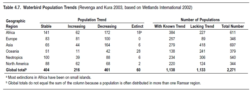
Trends in bird populations more generally have been best documented in Europe, North America, and Australia. In Europe, trend data are available from the Pan-European Common Bird Monitoring Scheme, currently implemented in 18 countries (Gregory et al. 2003). The data show trends in common in widespread farmland and woodland birds since 1980. (See Figure 4.17.) On average, populations of woodland birds in Europe have remained stable over the last 20 years, although their numbers have fluctuated in response to winter conditions (trend 1980– 2002 = -2%). Populations of common and widespread farmland birds, in contrast, have declined sharply, especially in the 1980s, and the downward trend continues at a slower rate (trend 1980– 2002 = -29%). This rapid decrease is believed to reflect a severe deterioration in the quality of farmland habitats in Europe, affecting both birds and other elements of biodiversity.

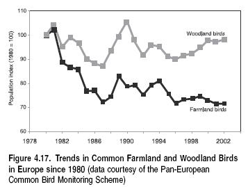
In Central and South America, where population-level data on bird species are scarce, BirdLife International has devised a different approach to measuring the decline in species richness. In Figure 4.18 (in Appendix A), a density map depicts the areas where threatened bird species used to occur but now no longer do so (mapped at a resolution of 1/4 degree grid cell) (BirdLife 2004b). This measures a decline in occupancy (measured as a decline in extent of occurrence), a variable typically correlated to abundance (Brown 1984; He and Gaston 2000). In the Neotropics, some 230 globally threatened birds—approximately 50% of threatened species that occur in the region—have become extinct across significant parts of their range. (This high proportion is not surprising, as many threatened species are classified as so based on declining trends in their ranges/populations (IUCN 2001)). On average, approximately 30% of their total ranges has been lost, varying from tiny areas of less than 100 square kilometers (approximately 40 species) to considerable areas of greater than 20,000 square kilometers (approximately 70 species).

This analysis is based on a review of areas or sites where species were recorded historically but not recently, or where habitat loss or other threats seem certain to have resulted in their disappearance. In some areas, up to 20 species have disappeared—the highest recorded density of local extirpations of globally threatened bird species in the world. Losses of range are inevitably associated with a reduction in the total numbers of individuals and hence, an increasing risk of extinction.

4.4.1.2 Mammals

Global estimates of changes in populations exist for many mammals. Ceballos and Ehrlich (2002) used a dataset consisting of all ranges of terrestrial mammals of Australia and subsets of ranges for terrestrial mammals of Africa, South East Asia, Europe, and North and South America, consisting of roughly 4% of about 4,650 known mammal species to compare historic and present ranges. In their sample, declining mammal species had collectively lost 50% of their continental populations as judged by loss in area. In Australia, where the data were most comprehensive, the proportion of declining species was 22%. The greatest population declines occurred in northeastern Australia and Tazmania. (See Figure 4.19.) If this were representative of all regions, it would suggest a greater than 10% loss of mammal populations. However, this may not be indicative of other areas, as Australian mammals have been among the most prone to extinction (Hilton-Taylor 2000).

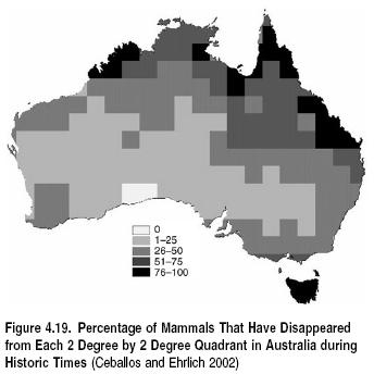
There are a few important datasets on population trends in large mammals. For example, the IUCN Species Survival Commission has monitored trends in rhinoceros populations in Africa and Asia for over 20 years (Khan 1989; Cumming et al. 1990; Foose and van Strien 1997; Emslie and Brooks 1999). This dataset reveals highly divergent trends between the different rhinoceros species. Two species, the southern white rhinoceros (Ceratotherium simum simum) and the Indian rhinoceros (Rhinoceros unicornis), have experienced long-term increases for the last century under very strict conservation and management regimes, whereas the black rhinoceros (Diceros bicornis), northern white rhinoceros (C. simum cottoni), and the Sumatran rhinoceros (Dicerorhinus sumatrensis) have suffered from catastrophic declines, mainly due to illegal hunting. In the case of the black rhinoceros, intensive conservation measures have stabilized the situation since the early 1990s. For the northern white rhinoceros and the Javan rhinoceros (R. sondaicus), the trends are uncertain (both have perilously small populations).

Whale populations are monitored by the Scientific Committee of the International Whaling Commission. Their data indicate significantly increasing population trends for four whale stocks involving three species: gray whale Eschrichtius robustus eastern north Pacific; bowhead whale Balaena mysticetus Bering-Chukchi- Beaufort Seas stock; humpback whale Megaptera novaeangliae western north Atlantic; and humpback whale M. novaeangliae Southern Hemisphere south of 60^o S in summer. These increasing trends reflect population recoveries following a period of very heavy harvesting pressure; at present, the datasets are not available to compare current whale population levels with historical estimates (although recalculation of the whaling commission’s catch data might make this possible in the future). So although these data indicate some recovery in certain whale populations, it is in the context of major overall declines since the onset of commercial whaling. Recent analyses based on genetic markers indicate that these declines may have been even more dramatic than previously thought (Roman and Palumbi 2003).

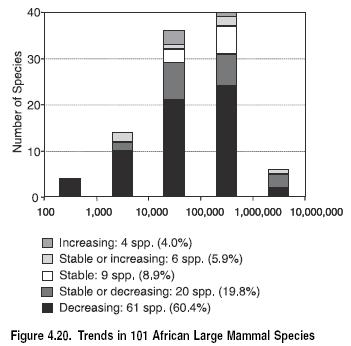
While there are few strictly freshwater mammal species, some are considered freshwater system–dependent or semi-aquatic mammals, given that they spend a considerable amount of time in fresh water. Unfortunately, population trend data on most of these species are lacking, but information does exist for some well-studied species (such as the pygmy hippopotamus and some otter populations in Europe) (Revenga and Kura 2003). A group for which there is more information on population trends, given their precarious conservation status, is the freshwater cetaceans or river dolphins. There are five species of river dolphins and one species of freshwater porpoise living in large rivers in Asia and South America. Populations of river cetaceans have declined rapidly in recent years, driven by habitat loss and degradation (Reeves et al. 2000).

While trends in populations of single species or small taxonomic groups provide useful information, multispecies datasets are more useful for identifying general overall trends. In Figure 4.20, trend data from various IUCN/SSC sources have been assembled into trend categories (reflecting changes over the last 20 years) in order to provide an overall picture of population or abundance trends among 101 large mammal species in Africa (data provided courtesy of the IUCN/SSC, with particular reference to Oliver 1993; Nowell and Jackson 1996; Oates 1996; Sillero-Zubiri and Macdonald 1997; Woodroffe et al. 1997; Mills and Hofer 1998; Barnes et al. 1999; East 1999; Emslie and Brooks 1999; Moehlman 2002). From this figure, it can be seen that over 60% of the species are clearly decreasing, and another almost 20% are in the ‘‘stable or decreasing’’ category. Only 4% of the species are clearly increasing. The Figure also shows that a larger fraction of the species with smaller populations is declining than those with larger populations. This overall heavily negative trend is likely to be indicative of a deteriorating environmental situation over much of the African continent.

4.4.1.3 Amphibians

Populations of many amphibians are declining in several parts of the globe. Different possible causes have been suggested, including habitat change (mainly affecting small-scale freshwater habitats such as ponds and [[stream]s]), disease, climate change, acid precipitation, habitat loss, and increased UV-B irradiation. Houlahan et al. (2000) used data from 936 populations to examine global trends in amphibian populations. The studies that were analyzed ranged from 2 to 31 years in duration. Their findings suggest a relatively rapid decline from the late 1950s peaking in the 1960s, followed by a reduced decline to the present. Alford et al. (2001) later reanalyze the same data and suggested that the global decline may have begun in the 1990s.

Regardless of the exact timeframe, it is commonly accepted that amphibian populations have recently declined on a global scale. This is supported by the recent IUCN-SSC/CI-CABS/ NatureServe Global Amphibian Assessment (Stuart et al. 2004). Out of the 4,048 amphibian species (70.9%) for which trends have been recorded, 61.0% (2,468 species) are estimated to be declining, 38.3% (1,552 species) are stable, and 0.69% (28 species) are increasing (Baillie et al. 2004). The report estimated that there are presently 435 more amphibians listed in the IUCN higher categories of threat then would have been in 1980 and that between 9 and 122 species have gone extinct during this time period (Stuart et al. 2004).

4.4.1.4 Reptiles

Global trends in reptiles have not been synthesized to the same extent as they have for amphibians. The fact that IUCN has only assessed the conservation status of 6% of the 8,163 described reptiles indicates how little is known about their global status and trends (Baillie et al. 2004). Reptiles share many of the same environments and are susceptible to many of the same threats as amphibians, and it has therefore been suggested that they may be experiencing similar or greater declines (Gibbins et al. 2000), but this remains to be rigorously tested.

Turtles and tortoises are among the best-studied reptiles. Within this group, large declines have been identified in the marine turtles, with six of the seven species listed as threatened by IUCN (Baillie et al. 2004). Overall rates of decline are unknown for turtles and tortoises, but reports on the trade of Southeast Asian freshwater turtles indicate that many of these species are rapidly declining. TRAFFIC Southeast Asia estimates trade volumes at a minimum of 13,000 tons of live turtles in 1999 (TRAFFIC Southeast Asia 2001, see section 5.4.5) and that this trade is increasing. IUCN is now conducting a Global Reptile Assessment that will soon help clarify the status and trends of this group.

4.4.1.5 Fish

Little is known about the majority of fish populations, but the global decline of commercially important fish stocks or populations is relatively well documented (e.g., Jackson et al. 2001; Myers and Worm 2003; Hutchings and Reynolds 2004).

Data on trends of some 600 fish populations covering more than 100 species can be found at fish.dal.ca/ to myers/data.html, usually in terms of trends in spawning stock biomass. Summarized data on the overall status of fish stocks, based on catch statistics in their SOFIA report, are available from FAO in The State of the World’s Fisheries and Aquaculture reports produced every two years (see FAO 2000a).

The data available to FAO at the end of 1999 identified 590 ‘‘stock’’ items. For 441 (75%) of these, there is some information on the state of the stocks and, although not all of this is recent, it is the best that is available. The stock items are classified as underexploited (U), moderately exploited (M), fully exploited (F), overexploited (O), depleted (D), or recovering (R), depending on how far they are, in terms of biomass and fishing pressure, from the levels corresponding to full exploitation. Full exploitation is taken as being loosely equivalent to maximum sustainable yield (equivalent to being harvested at the biological limit). The overall state of the fish stocks being monitored according to these classifications is shown in Figure 4.21.

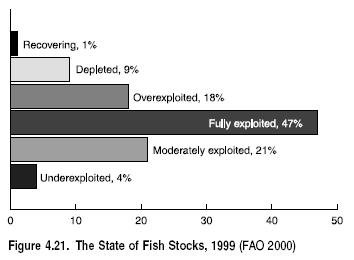
Figure 4.21 indicates that 28% (R+D+O) of the fish stocks being assessed have declined to levels below which a maximum sustainable yield can be taken and that a further 47% (F) require stringent management (which may or may not already be in place) to prevent decline into a similar situation. In total, 75% of these stocks (R+D+O+F) need management to prevent further declines or to bring about recovery in spawning stock biomass. Conversely, 72% (F+M+U) of the stocks are still capable of producing a maximum sustainable yield. These data have also been broken down regionally and are available in FAO (2002).

The State of the World’s Fisheries and Aquaculture report (FAO 2000a) identifies trends since 1974 in each stock classification, as a percentage of the total number of fish stocks being assessed by FAO. The percentage of underexploited stocks (U+M) has declined steadily, while the proportion of stocks exploited beyond maximum sustainable yield levels (O+D+R) has increased steadily over this time period. If these data are representative of fisheries as a whole, they indicate an overall declining trend in spawning stock biomass for commercially important fish species over the last 30 years.

The FAO data (FAO 2000a) demonstrate that there is significant increase in the exploitation of deep-sea fish stocks, such as populations of orange roughy (Hoplostethus atlanticus), alfonsinos (Berycidae), and dories (Zeidae). Many of these species have slow growth rates, and it is not yet clear that the methods established to fish them sustainably will be successful.

Little is known about the status of most shark populations (Castro et al. 1999). Baum et al. (2003) used the largest shark dataset covering the north Atlantic to assess declines of coastal and oceanic shark populations. Shark declines are believed to be occurring as a result of increased bycatch from pelagic long-line fisheries (Fisheries and aquaculture) and direct exploitation for shark fins. Baum et al. (2003) found that all recorded shark species within the study area, with the exception of makos, have experienced a decline of more than 50% in the past 8–15 years. Sharks grow and reproduce slowly, so even if exploitation were stopped, their recovery would be slow.

The use of catch statistics to assess freshwater stocks, which is common practice with marine species, is difficult because much of the inland catch is underreported by a factor of three or four, according to FAO (FAO 1999; FAO 2000a). Nevertheless, FAO’s last major assessment of inland fisheries (FAO 1999) reported that most inland capture fisheries that rely on natural reproduction of the stocks are overfished or are being fished at their biological limit.

Some large lakes have been systematically studied because of their importance as a fishery resource. The North American Great Lakes are a case in point. Annual fish stock assessments are conducted for commercially important salmonoid species, such as lake trout and Pacific salmon, and for their prey species (such as alewife, rainbow smelt, bloater, sculpin, and lake herring) (USGS Great Lakes Science Center 2003). The prey population assessments for the five lakes show that with the exception of Lake Superior, whose status is mixed but improving, populations of prey species in the other four lakes are all decreasing (USGS Great Lakes Science Center 2003). With respect to predator species in the lakes, many native species, such as lake trout and sturgeon, are found in vastly reduced numbers and have been replaced by introduced species (Environment Canada and U.S. EPA 2003).

Other regularly assessed lakes include Lake Victoria and Lake Tanganyika in Africa. These also show a decline in native fisheries and replacement with exotic species. The most widely known and frequently cited is the disappearance of over 300 haplochromine cichlids in Lake Victoria and the decline or disappearance of most of the riverine fauna in the east and northeastern forests of Madagascar (Stiassny 1996). There is also documented evidence of the threatened fish fauna of crater lakes in western Cameroon and the South African fish fauna, which has 63% of its species endangered, threatened, or ‘‘of special concern’’ (Moyle 1992; Lévêque 1997).

The few examples of riverine fish [[assessment]s] show that many inland fisheries of traditional importance have also declined precipitously. The European eel fishery, for example, has steadily declined over the last 30 years (Kura et al. 2004). By the mid-1980s, the number of new glass eels (eel juveniles) entering European rivers had declined by 90%. Recent figures show that this has now dropped to 1% of former levels (Dekker 2003).

Other fish stocks for which there is longer-term catch and status information include Pacific and Atlantic salmon in North America, fisheries of the Rhine and Danube Rivers in Europe, and fisheries of the Pearl River in China. All of these have declined to just a small fraction of their former levels due to overexploitation, river alteration, and habitat loss, putting some of these species at serious risk of extinction (Balcalbaca-Dobrovici 1989; Lelek 1989; Liao et al. 1989; WDFW and ODFW 1999).

Finally, even fisheries that until recently were reasonably well managed, such as the caviar-producing sturgeons in the Caspian Sea, and fisheries from relatively intact rivers such as the Mekong in Southeast Asia are rapidly declining (Kura et al. 2004.). For example, while almost all 25 species of sturgeon in the world have been affected to some degree by habitat loss, fragmentation of rivers by dams, pollution, and overexploitation, much of the recent decline in the catch of caviar-producing sturgeon is a direct result of overfishing and illegal trade (De Meulenaer and Raymakers 1996; WWF 2002). Major sturgeon populations have already declined by up to 70% (WWF 2002).

4.4.1.6 Corals

A meta-analysis of trends in Caribbean corals reveals that there has been a significant decline over the past three decades and although the decline has slowed, the trend persists. The average hard coral cover on reefs has been reduced by 80%, from around 50% to 10% cover, in three decades (Gardner et al. 2003). This significant trend supports the notion that coral reefs are globally threatened (Hodgson and Liebeler 2002; Hughes et al. 2003). (See Chapter 19.)

4.4.1.7 Invertebrates

Invertebrates represent the greatest proportion of eukaryotic biodiversity, but we know virtually nothing about their distributions, populations, or associated trends. However, especially among the insects a few well-studied groups such as butterflies, moths, and dragonflies (Hilton-Taylor 2000) may provide some insight. One example—a regional study of butterflies in the Netherlands (van Swaay 1990)—identifies decline as the most common trend over the past century. Of the 63 species assessed, 29 (46%) decreased or became extinct, 17 (27%) experienced little change, and 7 (11%) appeared to have increased their range. The remaining 10 species (16%) tended to fluctuate in range. Butterflies have also been relatively well monitored in the UK. Although many common and widespread species are believed to have increased in range and abundance (Pollard et al. 1995), the overall trend appears to be one of decline. A recent study examining population and regional extinctions indicates that British butterfly distributions have decreased by 71% over the past 20 years (Thomas et al. 2004b). This was found to be much higher than both birds and plants.

Although trends of well-studied insects indicate that this group shows similar trends of decline to other taxonomic groups, some studies indicate that insects in specific habitat types may be relatively resistant (Karg and Ryszkowski 1996). Understanding the general trends associated with insects is extremely important as it will provide much greater insight into global trends in biodiversity.

Two other groups of invertebrates that have been studied in more detail are freshwater mollusks and crustaceans. There are many lists on freshwater mollusks at national and regional levels, a number of which are available on the Internet (e.g. species .enviroweb.org/omull.html and www.worldwideconchology .com/DatabaseWindow.html). These databases, however, are not standardized or comparable; therefore an assessment of the current status and trends of freshwater mollusks at the global level is difficult. Existing lists are also biased toward terrestrial and marine groups.

The United States is one of the few countries in which the conservation status of freshwater mollusks and crustaceans has been widely assessed. Half of the known U.S. crayfish species and two thirds of U.S. freshwater mollusks are at risk of extinction (Master et al. 1998), with severe declines in their populations in recent years. Furthermore, at least 1 in 10 of the freshwater mollusks is likely to have already gone extinct (Master et al. 1998). The alarming rate of extinction of freshwater mollusks in eastern North America is even more pronounced. According to the U.S. Federal Register, less than 25% of the present freshwater bivalves appear to have stable populations. The status of gastropods is much less known. Of 42 species of extinct gastropods in the United States, 38 were reported from the Mobile Bay Basin in Southern North America (Bogan 1997).

4.4.1.8 Plants

Information on global trends in the status of plants is lacking, but overall population declines are likely given the high rates of habitat modification and deforestation described earlier, along with other threats, such as overexploitation, alien invasive species, pollution, and climate change. In addition, 12 of the 27 documented global extinctions over the past 20 years have been plants (Baillie et al. 2004).

The sixth meeting of the Conference of the Parties of the Convention on Biological Diversity adopted the Global Strategy for Plant Conservation. This strategy highlights monitoring (Environmental monitoring and assessment) the status and trends of global plant diversity as one of the objectives (UNEP 2002b), which it is hoped will lead to greater insight into global trends.

Cycads are one of the few groups where the conservation status of all species has been assessed and trend data exist. Population trends are available for 260 species of cycads (Cycadopsida, 288 species in total). Of these, 79.6% (207 species) are declining, 20.4% (53 species) are stable, and none are considered to be increasing (Baillie et al. 2004).

Another important dataset is available for trends in wood volume and biomass. FAO’s Forest Resources Assessment 2000 indicates opposing trends between the tropics and nontropics in terms of both volume and above-ground woody biomass over the period 1990–2000. There has been a decreasing trend in the tropics, compared with an increasing trend in the nontropics. These data should be interpreted with caution, due in part to problems of data compatibility between countries (see FAO 2001b and Chapter 21 for more details). Note also that no distinction is made here between undisturbed forest, secondary forests, and plantations.

4.4.1.9 Conclusion on Population

Measuring change in populations is important for understanding the link between biodiversity and ecosystem function, as significant changes in populations can have important implications for the function of ecosystems long before any species actually goes extinct (e.g., Jackson et al. 2001; Springer et al. 2003).

The data presented in this section represent a brief assessment of the types of data that are available on the trends in populations. Although the datasets described are not easily comparable with each other and are certainly not collectively representative of biodiversity as a whole, a few basic conclusions can be drawn.

Both declining and increasing trends can be documented from available studies; in most cases, declining trends appear to outweigh increasing trends, often by a considerable margin, and some increasing trends can be related to very specific situations (for example, population recovery following periods of intensive harvesting or successful reintroduction programs). Overall, the emerging evidence suggests that for macroorganisms, especially those with small areas of distribution, most populations are declining as a result of human activities and are being replaced by individuals from a much smaller number of expanding species that thrive in human-altered environments. The result will be a more homogenized biosphere with lower diversity at regional and global scales (McKinney and Lockwood 1999).

4.4.2 Species

4.4.2.1 Current Extinction Rates

The evolution of new species and the extinction of others is a natural process. Species present today represent only 2–4% of all species that have ever lived (May et al. 1995). Over geological time there has been a net excess of speciation over extinction that has resulted in the diversity of life experienced today. However, the high number of recent extinctions suggests that the world might now be facing a rapid net loss of biodiversity. This can be tested by comparing recent extinction rates to average extinction rates over geological time.

The fossil record appears to be punctuated by five major mass extinctions (Jablonski 1986), the most recent of which occurred 65 million years ago. However, the majority of extinctions have been spread relatively evenly over geological time (Raup 1986), enabling estimates of the average length of species’ lifetimes through the fossil record. Studies of the marine fossil record indicate that individual species persisted for periods ranging from 1 million to 10 million years (May et al. 1995). These data probably underestimate background extinction rates, because they are necessarily largely derived from taxa that are abundant and widespread in the fossil record.

Using a conservative estimate of 5 million as the total number of species on the planet, we would therefore expect anywhere between five extinctions per year to roughly one extinction every two years (for all 5 million species on the planet). As noted earlier, recent extinctions have been best studied for birds, mammals, and amphibians, and in these groups over the past 100 years roughly 100 species have become extinct. This is in itself similar to background extinction rates, but these groups represent only 1% of described species.

Assuming for the moment that the susceptibility to extinction of birds, mammals, and amphibians is similar to species as a whole, then 100 times this number of species (10,000 species) were lost over the past 100 years. But this assumption of equivalent extinction risk is very uncertain, and given the additional uncertainty over the total number of species on the planet, it is preferable to convert these data into a relative extinction rate, measured as the number of extinctions per million species per year (Pimm et al. 1995). A background extinction rate of 0.1–1 E/MSY then corresponds to the average marine fossil species lifetimes. Mammalian background extinction rates are also believed to be within these limits, falling within a range of 0.21 E/MSY (strictly for lineages rather than species, but provides a conservative estimate (Alroy 1998; Regan et al. 2001) and 0.46 E/MSY (Foote 1997).

Measuring recent extinction rates is difficult, not only because our knowledge of biodiversity is limited, but also because even for the best studied taxa there is a time lag between the decline toward extinction and the actual loss of species. In the case of extinctions caused by habitat loss, in particular, it may take thousands of years before a restricted remnant population is finally driven to extinction (Diamond 1972).

With this in mind, it is possible to use recent documented extinctions to make a very conservative estimate of current extinction rates, though this is limited because only a few taxonomic groups have been reasonably well analyzed for extinctions. There are approximately 21,000 described species of birds, mammals, and amphibians. The roughly 100 documented extinctions for these groups during the past century yields an E/MSY of 48, which is 48 to 476 times greater than the background extinction rate of 0.1 to 1. If ‘‘possibly extinct’’ species are included in this analysis, the total number of extinctions and possible extinctions over the past 100 years for these groups is 215 species, which results in an E/MSY that is 102 to 1,024 higher than background rates. Broken down by taxonomic group, mammals have the highest E/MSY (64) followed by birds (at 45) and finally amphibians (40). If possibly extinct species are considered, however, then amphibians have the highest E/MSY at 167 followed by mammals with 68 and finally birds with 59. (It should be noted that mammals have not been completely assessed for possibly extinct species (see Baillie et al. 2004).)

A broad range of techniques have been used to estimate contemporary extinction rates, including estimates based on both direct drivers (such as habitat destruction) and indirect drivers (such as human energy consumption) of extinction (Myers 1979; Myers 1988; Reid 1992; Smith et al. 1993; Ehrlich 1994; Mace and Kunin 1994; Pimm and Brooks 1999; Regan et al. 2001; Baillie et al. 2004; also see MA Scenarios, Chapter 10). Many of these studies give rise to estimates of E/MSY that are 1,000 to 10,000 higher than background rates (Pimm and Brooks 1999), generally higher than the conservative estimate for birds, mammals, and amphibians based on documented extinctions. (See Figure 4.22 in Appendix A.) Estimates based on documented extinctions are likely to be underestimates because the IUCN Red List is very conservative in recording species as actually extinct and because many extinctions have probably been missed due to limited survey effort for most taxonomic groups.

The trend in species extinction rates can be deduced by putting together extinction rates characteristic of well-recorded lineages in the fossil record, recorded extinctions from recent times, and estimated future extinction rates based on the approaches just described. All these estimates are uncertain because the extent of extinctions of undescribed species is unknown, because the status of many described species is poorly known, because it is difficult to document the final disappearance of very rare species, and because there are extinction lags between the impact of a threatening process and the resulting extinction (which particularly affects some modeling techniques). However, the most definite information, based on recorded extinctions of known species over the past 100 years, indicates extinction rates are around 100 times greater than rates characteristic of comparable species in the fossil record. Other less direct estimates, some of which refer to extinctions hundreds of years into the future, estimate extinction rates 1000 to 10,000 times higher than rates recorded among fossil lineages.

Current anthropogenically caused extinction is not solely a characteristic of contemporary societies. Since the initial revelations that humanity greatly inflated extinction rates with stoneage technology (Martin and Wright 1967; Martin and Klein 1984), large quantities of new data have demonstrated significant extinction episodes occurred with, for example, the arrival of people in Australia 46,000 years ago (Roberts et al. 2002), in the Americas 12,000 years ago (Alroy 2001), in Madagascar (Goodman and Patterson 1997) and the Pacific 2,000 years ago (Steadman 1995), and elsewhere (MacPhee 1999).

4.4.2.2 Current Levels of Threat to Species

At a global level, nearly 850 species have been recorded as becoming extinct or at least extinct in the wild since 1500 (Baillie et al. 2004). Species extinctions represent the final point in a series of population extinctions; in fact, distinct populations may be being lost at a rate much faster than species overall, with serious negative consequences for local ecosystem function (Hughes et al. 1997).

The most extensive global dataset on trends in species richness is the IUCN Red List of Threatened Species (see www.redlist.org and Baillie et al. 2004). The IUCN Red List is formalized through the application of categories and criteria (IUCN 2001) that are based on assessments of extinction risk (Mace and Lande 1991). These criteria are now broadly used in many parts of the world and have been adapted for use at multiple scales.

The 2004 IUCN Red List of Threatened Species is based on assessments of 38,047 species. Of these, 7,266 animal species and 8,321 plant species (15,547 species in total) have been placed in one of the IUCN Categories of Threat (vulnerable, endangered, or critically endangered). However, the IUCN Red List needs to be interpreted with caution, because for most taxonomic groups the assessments are very incomplete and heavily biased toward the inclusion of the most threatened species. As of 2004, assessments of almost every species have been completed for three animal groups (mammals, birds, and amphibians) and two plant groups (conifers and cycads). The number of species in each IUCN Red List Category for all five of these groups is given in Table 4.8. Reptiles have not yet been completely assessed.

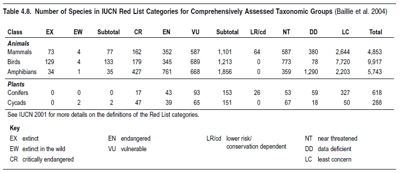
In all five of these groups, the proportions of species in categories of high extinction risk are much greater than would be expected if species were becoming extinct at rates typically observed over geological time. The levels of threat are lowest among birds, where 12% of species are threatened (vulnerable+endangered +critically endangered). There has been a trend of increasing threat between 1988 and 2004, as measured by the movement of species into more threatened Red List Categories (BirdLife 2004b). The relatively low level of threat in birds is possibly related to their tendency to be highly mobile, resulting in their generally wide geographic distributions.

The pattern of distribution of threat categories among species is broadly similar for mammals and conifers, with 23% (1,101) and 25% (153) respectively of the species being globally threatened. Based on the evidence from comprehensive regional assessments (e.g., Stein et al. 2000), it is more than possible that future studies will show this very high level of threat to be typical of the current global situation among most groups of terrestrial species.

The situation with amphibians is broadly similar: 32% (1,856) globally threatened. However, the true level of threat among amphibians is probably masked by the fact that 23% of the species are classified as data-deficient (compared with 8% for mammals and 10% for conifers). The overall conservation situation of amphibians will probably eventually prove to be much worse than the mammal and conifer situations and might be typical of the higher levels of threat associated with freshwater (or freshwater-dependent) species (Master et al. 2000). Amphibian extinction risk has been retrospectively analyzed back to the early 1980s, and shows a similar rate of decline to that of birds (BirdLife 2004b), but with a greater number of the more seriously threatened species declining (Baillie et al. 2004).

The cycad situation is much worse, with 52% (151) of species globally threatened. This is possibly reflective of the relict nature of these ancient species, with most species now surviving only in very small populations.

Species are not all equal: some represent much more evolutionary history than others (Vane-Wright et al. 1991). If extinctions were randomly distributed across the tree of life, surprisingly little evolutionary history would be lost (Nee and May 1997). However, extinctions are far from phylogenetically random: there is strong taxonomic selectivity in the current extinction crisis, with the result that the loss of evolutionary history is much more than that expected were species to be lost randomly with respect to their taxonomic affiliation (Purvis et al. 2000a).

There is a clear trend for higher levels of threat among the larger species. Of the mammals, for example, 38% (81) of the Artiodactyla (antelopes, cattle, sheep, and so on), 82% (14) of the Perissodactyla (horses, rhinos, and tapirs), 39% (114) of the Primates, 100% (2) of the Proboscidea (elephants), and 100% (5) of Sirenia (dugongs and manatees) are globally threatened (Baillie et al. 2004). Among the birds, high levels of threat are particularly apparent among orders such as Apterygiformes (kiwis) with 100% (4) threatened, Sphenisciformes (penguins) 57% (10), Pelecaniformes (cormorants, pelicans, and so on) 26% (17), Procellariiformes (albatrosses and petrels) 47% (62), Ciconiiformes (storks, ibises, and spoonbills) 21% (28), Galliformes (pheasants, partridges, quails, and so on) 27% (78), Gruiformes (cranes, bustards, rails, and so on) 33% (76), Columbiformes (doves and pigeons) 22% (75), and Psittaciformes (parrots) 29% (109) (Baillie et al. 2004). These orders include species that are flightless, ground-dwelling, particularly vulnerable to alien predators, and edible or economically valuable. The most noteworthy result from the threat analysis of amphibians is the particularly large proportion of globally threatened salamanders—46% (234) of the total number of threatened amphibians. Salamanders are often long-lived, slow-breeding species, with limited ability to disperse over significant distances.

The IUCN Red List does not yet include comprehensive datasets for taxonomic groups confined to [[freshwater (Freshwater biomes)] ecosystems]. Nor have there been any complete assessments of any invertebrate groups. Some important regional datasets are becoming available, however, for example for North America, compiled by NatureServe. A summary and analysis of these data for the United States are presented in Stein et al. (2000). NatureServe uses a different system for categorizing levels of threat, and their categories are not strictly comparable with those of IUCN. Nevertheless, for the purposes of this assessment their system does broadly indicate levels of extinction risk and is therefore useful in determining trends.

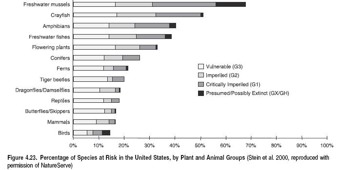
Based on an assessment of 20,439 species, NatureServe determined that one third of the U.S. flora and fauna appears to be of conservation concern. NatureServe has comprehensively assessed the status of every U.S. species in 13 taxonomic groups, and the percentage of each of these species that is at risk is shown in Figure 4.23. The most noteworthy finding of this study is that the species groups relying on freshwater habitats—mussels, crayfishes, stoneflies, fishes, and amphibians—exhibit the highest levels of risk. Sixty-nine percent of freshwater mussels are at risk. Dragonflies and damselflies seem to be an exception to this pattern since, despite being freshwater-dependent, their threat level is relatively low. The threat levels are also very high in the United States for flowering plants (33%).

No comprehensive assessment has yet been carried out on the threat levels for any marine group. However, work is progressing fast to assess the status of all the chondrichthyan fishes (sharks, rays, and chimaeras). To date, the IUCN/SSC Shark Specialist Group has assessed one third (373 species) of the world’s chondrichthyans (out of a total of approximately 1,100 species), and 17.7% are listed as threatened (critically endangered, endangered, or vulnerable), 18.8% near-threatened, 37.5% data-deficient, and 25.7% of least concern (Baillie et al. 2004). However, it is not at all clear that sharks and rays are good indicators of overall biodiversity trends in [[marine] ecosystems]. In view of the life history strategies for these species (slow-breeding, long-lived), it is likely that they are more threatened than some other marine groups.

4.4.2.3 Traits Associated with Threat and Extinction

The patterns of threat and extinction are not randomly distributed among species (Bennett and Owens 1997; Gaston and Blackburn 1997b; Owens and Bennett 2000). Ecological traits demonstrated to be associated with high extinction risk (even after controlling for phylogeny) include high trophic level, low population density, slow life history or low fecundity, and small geographical range size (Bennett and Owens 1997; Purvis et al. 2000b). For primates and carnivores, these traits together explain nearly 50% of the total between-species variation in extinction risk, and much of the remaining variation can be accounted for by external anthropogenic factors that affect species irrespective of their biology (Purvis et al. 2000b).

However, different taxa are threatened by different mechanisms, which interact with different biological traits to affect extinction risk. For bird species, extinction risk incurred through persecution and introduced predators is associated with large body size and long generation time but is not associated with degree of specialization, whereas extinction risk incurred through habitat loss is associated with habitat specialization and small body size but not with generation time Owens and Bennett (2000). For Australian marsupials, the risk of extinction has been found to be better predicted by geographical range overlap with sheep (Fisher et al. 2003).

Extinction risk is not independent of phylogeny, presumably because many of the biological traits associated with higher extinction risk tend to co-occur among related species. Among birds, for example, families that contain significantly more threatened species than average are the parrots (Psittacidae), pheasants and allies (Phasianidae), albatrosses and allies (Procellariidae), rails (Rallidae), cranes (Gruidae), cracids (Cracidae), megapodes (Megapodidae), and pigeons (Columbidae) (Bennet and Owens 1997). There is also a positive relationship between the proportion of species in a taxon that are considered to be threatened and the evolutionary age of that taxon, both for the global avifauna and the avifauna of the New World (Gaston and Blackburn 1997b).

The majority of recorded species extinctions since 1500 have occurred on islands. A total of 72% of recorded extinctions in five animal groups (mammals, birds, amphibians, reptiles, and mollusks) were of island species (Baillie et al. 2004). Island flora and fauna were especially vulnerable to the human-assisted introduction of predators, competitors, and diseases, whereas species on continents were not so ecologically naive. However, predictions of future extinctions stem from the ongoing loss of continental, tropical forests; hence 452 of a total of 1,111 threatened bird species are continental (Manne et al. 1999). A shift from island to mainland extinctions is consistent with a recent examination of extinctions over the past 20 years, where island and mainland extinctions were roughly equal (Baillie et al. 2004).

4.4.2.4 Geographical Patterns of Threat and Extinction

The geography of threat and extinction is far from even, with the majority of threatened species concentrated in tropical and warm temperate endemic-rich ‘‘hotspots’’ (Myers et al. 2000). Figure 4.24 shows the locations of known mammal, bird, and amphibian extinctions since 1500. The different patterns between these three groups are striking. Mammal extinctions are concentrated in the Caribbean and Australia. In both cases, these are thought to be second waves of human-induced extinction, following the overexploitation of the Pleistocene (MacPhee 1999); in any case, the current mammalian fauna in these regions is but a modest sample of the native fauna prior to human arrival, particularly in terms of medium- and large-sized mammals (Woods and Sergile 2001; Brook and Bowman 2004). The remainder of the recorded mammalian extinctions are widely scattered, most being on oceanic islands.

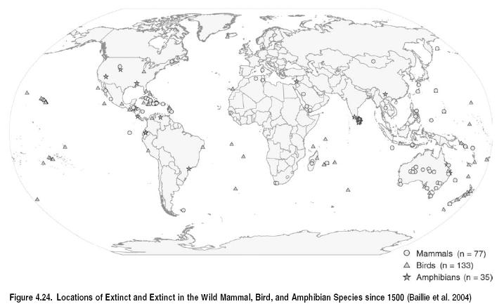
Avian extinctions are overwhelmingly concentrated on oceanic islands, especially on Hawaii and New Zealand (Steadman 1995), with very few elsewhere. With few exceptions, oceanic island avifaunas have lost most of their endemic species over the last 1,000 years.

The highest number of recorded amphibian extinctions is on Sri Lanka. However, the current wave of amphibian extinction, which appears to be accelerating, is concentrated in montane areas from Honduras south to northern Peru, in the Caribbean islands, in eastern Australia, and perhaps in the Atlantic Forest of southern Brazil.

Maps of species richness of threatened mammals and birds are presented in Figure 4.25 (in Appendix A). (For a species richness map of threatened amphibians, see Chapter 20.) The maps show interesting similarities and differences. They all show concentrations of threatened species in hotspots (Myers et al. 2000), in particular in the Andes, southern Brazil, West Africa, Cameroon, the Albertine rift of Central Africa, the Eastern Arc Mountains of Tanzania, eastern Madagascar, Sri Lanka, the Western Ghats of India, the eastern Himalayas, central China, mainland Southeast Asia, and Borneo.

The mammal map is noteworthy in that there is at least one threatened mammal species in most parts of the world. In addition to the geographic regions just listed, important concentrations of threatened mammals also occur in the eastern Amazon basin, southern Europe, Kenya, Sumatra, Java, the Philippines, and New Guinea. Interestingly, MesoAmerica, Australia, and the Caribbean islands appear to have relatively low numbers of threatened mammals. However, it should be noted that patterns of threat will appear low in areas where the vulnerable species have already gone extinct (which may be the case in the Caribbean and Australia) and that threatened mammals with extremely small distributions will not be easily viewed on the map (such as many restricted-range montane species in MesoAmerica).

The bird map differs in that the importance of oceanic islands is emphasized. Other areas that are of great importance for threatened birds but not listed earlier include the Caribbean islands, the Cerrado woodlands of Brazil, the highlands of South Africa, the plains of northern India and Pakistan, Sumatra, the Philippines, the steppes of central Asia, eastern Russia, Japan, southeastern China, and New Zealand. As with mammals, MesoAmerica and Australia are relatively unimportant for threatened birds. But so are the Amazon basin, Europe, Java, and New Guinea.

Amphibians generally have much more restricted ranges than birds and mammals (see Chapter 20), and threatened amphibian species therefore occupy a much smaller global area, a very different picture to mammals. In the small areas where they are concentrated, however, threatened amphibians occur more densely than either mammals or birds (up to 44 species per half-degree grid square, compared with 24 for both mammals and birds) (Baillie et al. 2004). The majority of the world’s known threatened amphibians occur from Mexico south to northern Peru and on the Caribbean islands. Most of the other important concentrations of globally threatened amphibians mirror the patterns of threat for mammals and birds, although eastern Australia and the southwestern Cape region of South Africa are also centers of threatened amphibians. The paucity of data from certain parts of the world probably results in serious underestimation of the concentrations of threatened amphibians, especially in the Albertine Rift, Eastern Himalayas, much of mainland Southeast Asia, Sumatra, Sulawesi, the Philippines, and Peru.

Lack of comprehensive geographic and threat assessment for other species groups precludes the presentation of maps for other taxa. Given the similarity between patterns of threatened species for mammals, birds, and amphibians, many other taxonomic groups such as reptiles, fish, invertebrates, and plants may demonstrate broadly similar patterns. However, there are also likely to be many differences. For example, distribution patterns of threatened reptiles (in particular, lizards) are likely to highlight the importance of many arid ecosystems. It is already known that some distribution patterns of threatened plants do not match those of most animal groups, the most notable examples being the Cape Floral Region and Succulent Karoo of South Africa and the deserts of the southwestern United States and northern Mexico. Patterns of threat in [[marine] ecosystems] will of course be completely different, and data on these patterns are still largely unavailable.

One potentially useful device for understanding variation in threat intensity across areas is the concept of extinction filters, whereby prior exposure to a threat selectively removes those organisms that are most vulnerable to it, leaving behind a community that is more resilient to similar threats in the future (Balmford 1996). This idea can explain temporal and spatial variation in species’ vulnerability to repeated natural changes in the past (such as glaciation events). It may also shed light on the contemporary and future impact of anthropogenic threats. For example, the impact of introduced rats on island-nesting seabirds appears less marked on islands with native rats or land crabs, which have selected for resilience to predators (Atkinson 1985). In a similar fashion, corals may be less likely to bleach in response to rising sea [[temperature]s] in areas where they have been repeatedly exposed to temperature stresses in the past (Brown et al. 2000; Podesta and Glynn 2001; West and Salm 2003).

One consequence of the global patterns of extinction and invasion is biotic homogenization. This is the process whereby species assemblages become increasingly dominated by a small number of widespread, human-adapted species. It represents further losses in biodiversity that are often missed when only considering local changes in absolute numbers of species. The many species that are declining as a result of human activities tend to be replaced by a much smaller number of expanding species that thrive in human-altered environments. The outcome is a more homogenized biota with lower diversity at regional and global scales. One effect is that in some regions where diversity has been low because of isolation, the biotic diversity may actually increase— a result of invasions of non-native forms (for example, some continental areas such as the Netherlands as well as oceanic islands). Recent data also indicate that the many losers and few winners tend to be nonrandomly distributed among higher taxa and ecological groups, enhancing homogenization.

4.4.2.5 Conclusion on Species

The rate of species extinction is several orders of magnitude higher than the natural or background rate, even in birds, where the level of threat is the lowest among the assessed taxa. And the great majority of threatened species continue to decline. The geography of declines and extinctions is very uneven and concentrated in particular areas, especially in the humid tropics. Past geographic extinction patterns vary markedly between mammals, birds, and amphibians, but future patterns (as indicated by patterns of currently threatened species) are likely to be more closely correlated. The limited data that exist suggest that biodiversity is more severely threatened in [[freshwater (Freshwater biomes)] ecosystems] than in [[terrestrial] ecosystems]. Studies suggest that ancient taxonomic lineages are particularly prone to extinction (Gaston and Blackburn 1997b; Purvis et al. 2000a). Biodiversity trends in [[marine] ecosystems] are yet to emerge, although from the limited data available, it appears that the general trends are not fundamentally different from those in terrestrial ecosystems.

4.4.3 Biomes

Rates of loss of natural land cover for the world’s [[biome]s] can be measured using a unique dataset on land use change, the HYDE dataset (Klein Goldewijk 2001). This dataset uses information on historical population patterns and agriculture statistics to estimate habitat conversion between 1950 and 1990, based on maps of 0.5-degree resolution. These data indicate that by 1950 all but two biomes (boreal forests (Forest biome) and tundra) had lost substantial natural land cover to croplands and pasture. (See Figure 4.26.) Mediterranean forests (Forest biome) and temperate grassland biomes had experienced the most extensive conversion, with roughly only 30% of native vegetation cover remaining in 1950.

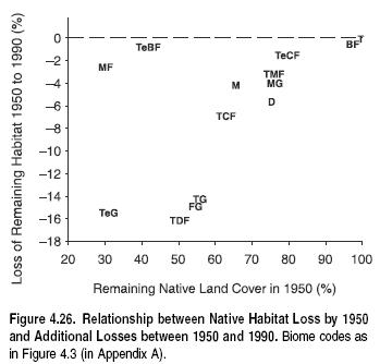
Loss of native habitat cover has continued, with most biomes experiencing substantial additional percentages of native land cover between 1950 and 1990. The tropical dry broadleaf forests biome has lost the highest percentage of additional habitat (16.1%); only tundra has lost very little if anything to agricultural conversion in those 40 years.

The percentage of remaining habitat in 1950 is highly correlated with rates of additional loss since then. This result indicates that, in general, patterns of human conversion among biomes have remained similar over at least the last century. For example, boreal forests had lost very little native habitat cover through until 1950 and have lost only a small additional percentage since then. In contrast, the temperate grasslands biome had lost nearly 70% of its native cover by 1950 and has lost an additional 15.4% since then. Two biomes appear to be exceptions to this pattern: Mediterranean forests and temperate broadleaf forests. Both of these biomes had lost the majority of their native habitats by 1950 but since then have lost less than 2.5% further habitat. These biomes contain many of the world’s most established cities and most extensive surrounding agricultural development (Europe, the United States, the Mediterranean basin, and China). It is possible that in these biomes the most suitable land for agriculture had already been converted by 1950.

In addition to the total amount of habitat loss, the spatial configuration of loss can strongly affect biodiversity. Habitat fragmentation typically accompanies land use change, leaving a complex landscape mosaic of native and human-dominated habitat types. Quantitative data on habitat fragmentation are difficult to compile on the scale of biomes or realms, but habitat fragmentation typically endangers species by isolating populations in small patches of remaining habitat, rendering them more susceptible to genetic and demographic risks as well as natural disasters (Laurance et al. 1997; Boulinier et al. 2001).

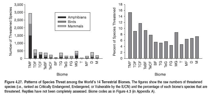
Changes in the biodiversity contained within the world’s biomes are generally assessed in terms of the species they contain. Changes in species, however, are difficult to measure. Species abundances can fluctuate widely in nature, making it difficult at times to detect a true decline in abundance. And, as described earlier, species extinctions are difficult to count, as the vast majority of species on Earth have yet to be described, extinctions are still relatively rare among known species, and establishing an extinction with confidence is difficult.

Given these difficulties, a reasonable indicator of current and likely future change in biodiversity within a biome is the number of species facing significant extinction risk. The threatened species identified by IUCN are used in this analysis. As such, the analysis is limited to terrestrial vertebrates, which represent less than 1% of the total species on Earth and may not fully represent patterns in other taxa.

Biomes differ markedly in the number of threatened species they contain (see Figure 4.27), with tropical moist forests housing by far the largest number. The percentage of total species that are endangered, however, is more similar among biomes with temperate coniferous forests approaching a similar percentage as tropical moist forests. Comparing these two patterns of threat suggests that higher absolute losses of species in tropical moist forests may be expected, with more similar rates of extinction in other biomes.

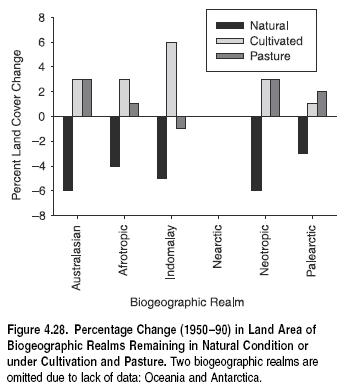
4.4.4 Biogeographic Realms

Like biomes, biogeographic realms differ markedly in the amounts of habitat conversion to agriculture before and since 1950. (Klein Goldewijk 2001). (See Figure 4.28.) By 1950, for example, the Indo-Malayan realm had already lost almost half its natural habitat cover. In all realms, at least a quarter of the area had been converted to other land uses by 1950. (These findings exclude Oceania and Antarctica due to lack of data.)

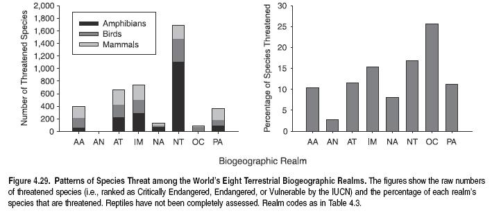
In the 40 years from 1950 to 1990, habitat conversion continued in nearly all biogeographic realms. More than 10% of the land area of the temperate northern realms of the Nearctic and Palearctic as well as the Neotropical realm has been converted to cultivation. Although these realms are currently extensively cultivated and urbanized, the amount of land under cultivation and pasture seems to have stabilized in the Nearctic, with only small increases in the Palearctic in the last 40 years. Within the tropics, rates of conversion to agriculture range from very high in the Indo-Malayan realm to moderate in the Neotropics and the Afrotropics, although land cover change has not yet stabilized and shows large increases, especially in cropland area since the 1950s. Australasia has relatively low levels of cultivation and urbanization, but these have also increased in the last 40 years.

As with biomes, the number of threatened vertebrate species differs widely among biogeographic realms (Baillie et al. 2004). (See Figure 4.29.) The largest numbers are found in tropical realms (Neotropic, Indo-Malay, and Afrotropic), while the Nearctic, Oceania, and Antarctica realms hold the least. The percentage of total species that are endangered, however, shows a very different pattern. Most strikingly, over 25% of species in Oceania are threatened, more than twice the percentage of any other realm. The high rates of species threat in Oceania are likely due to well-known factors that endanger island faunas, including high rates of endemism, severe range restriction, and vulnerability to introduced predators and competitors (Manne et al. 1999). Although the Neotropics contain many threatened species, the extraordinary richness of this realm results in a lower percentage of threatened species than Oceania. Therefore, based on species threat levels, we can expect a larger absolute change in biodiversity (measured as expected species extinctions) in the tropical continents, but the highest rates of extinction on tropical islands.

4.5 Improving Our Knowledge of Biodiversity Status and Trends

Biodiversity is a complex concept and so, therefore, is its measurement. Ideally, for any particular assessment, measures of biodiversity would reflect those aspects particularly relevant to the context (Royal Society 2003). For an assessment of ecosystem services for example, biodiversity assessment should be based on measures that are relevant to the provision of services and to human well-being. Unfortunately, the information currently available on global biodiversity is limited, and the data presented in this chapter are therefore rather general. As our understanding of the role of biodiversity improves, so does the potential for better and more relevant measures to be developed. This section considers the need for better indicators of biodiversity status and the specific context of indicators to measure progress against the 2010 biodiversity target, and some clear gaps that will have to be filled if we are to make progress in understanding trends in biodiversity and their consequences are highlighted.

4.5.1 Indicators of Global Biodiversity Status

Documenting trends in biodiversity and the actions and activities that affect it requires suitable indicators. Indicators in this sense are a scientific construct that uses quantitative data to measure biodiversity, ecosystem condition and services, or drivers of change. A useful indicator will provide information about changes in important processes, be sensitive enough to detect important changes but not so sensitive that signals are masked by natural variability, detect changes at the appropriate temporal and spatial scale without being overwhelmed by variability, be based on well-understood and generally accepted conceptual models of the system to which it is applied, be based on reliable data to assess trends and have a relatively straightforward data collection process, have monitoring (Environmental monitoring and assessment) systems in place for the underlying data needed to calculate the indicator, and be easily understood by policy-makers (NRC 2000 and see also Chapter 2 (Ecosystems and Human Well-Being: Volume 1: Current State and Trends: Biodiversity)).

Unfortunately, as noted earlier, most existing biological measures, especially those reflecting species richness or various aspects of [[species (Species diversity)] diversity], do not reflect many important aspects of biodiversity, especially those that are significant for the delivery of ecosystem services. In addition, few measures have been repeated to allow for a fair assessment of trends over time. Care also needs to be taken in the interpretation of these measures and their use as indicators. For example, these simple measures of species richness may not differentiate between native and invasive or introduced species, differentiate among species in terms of sensitivity or resilience to change, or focus on species that fulfill significant roles in the ecosystem (such as pollinators or decomposers). Moreover, many measures depend on the definition of the area and may be scale-dependent, and they may not always reflect biodiversity trends accurately.

Aggregate indicators of trends in species populations such as the Index of Biotic Integrity for aquatic systems (Karr and Dudley 1981) and the Living Planet Index (Loh and Wackermagel 2004; Loh et al. 2005) use published data on trends in populations of a variety of wild species to identify overall trends in species abundance and, by implication, the condition of the ecosystems in which they occur. The LPI can be applied at national, regional, and global levels, as described earlier. Although it is based on a large number of population trends, various sampling biases affect the index, though with care these biases can be addressed (Loh et al. 2005). Being based on local population abundances, the LPI may be an appropriate biodiversity indicator for ecosystem services, especially with careful sampling of the populations included in its calculation. A complementary index is the Red List Index derived from the IUCN Red List of threatened species (Butchart et al. 2004). Red List Indices illustrate the relative rate at which a particular set of species changes in overall threat status (that is, projected relative extinction-risk), based on population and range size and trends as quantified by Red List categories. RLIs can be calculated for any representative set of species that has been fully assessed at least twice. The RLI for the world’s birds shows that that their overall threat status has deteriorated steadily during 1988–2004 in all biogeographic realms and ecosystems. A preliminary RLI for amphibians for 1980–2004 shows similar rates of decline (Butchart et al 2005). Both these indexes (LPI and RLI) synthesize much detailed information into a few compelling data points and are being used for assessing progress against the Convention on Biological Diversity’s 2010 target.

Currently there has been much less attention paid to the development of indicators for aspects of biodiversity other than species and populations. One recent attempt to collate and synthesize all up-to-date estimates of global trends in population size or habitat extent could find global estimates of habitat change (spanning at least five years since 1992) for only four major [[biome]s] (tropical forest, temperate and boreal forest, seagrass, and mangroves) (Balmford et al. 2003a). Neither has there been a focused process to measure the intensity and trends in the key drivers of biodiversity change or the implementation and effectiveness of response options. (See Chapter 5 of the Policy Responses volume.) It is clear that a broader set of biodiversity indicators is required, with indicators that are aligned against valued aspects of biodiversity. The adoption of the 2010 biodiversity target makes this task still more urgent (Balmford et al. 2005; Green et al. 2005).

4.5.2 The CBD 2010 Biodiversity Target

In April 2002, at the Sixth Conference of the Parties of the Convention on Biological Diversity, 123 Ministers described a desire to halt biodiversity loss and further committed themselves to actions to ‘‘achieve, by 2010, a significant reduction of the current rate of biodiversity loss at the global, regional and national levels as a contribution to poverty alleviation and to the benefit of all life on earth’’ (Decision VI/26; CBD Strategic Plan). Carrying this message forward, the world’s leaders, at the World Summit on Sustainable Development, set a target for ‘‘a significant reduction in the current rate of loss of biological diversity’’ by 2010. This target has now been adopted formally by the parties to the CBD as well as by all participants in the WSSD. The same or a similar target is being adopted at regional levels. For example, the European Union Council adopted a more ambitious target and agreed in 2001 ‘‘that biodiversity decline should be halted . . . by 2010’’ (European Council 2001).

Apart from the data gathering needed to assess progress against the target, its formulation poses some technical challenges, especially for its implementation at a global level. First, the measures of biodiversity to be used as indicators need to be available over a sufficient time period, need to have been measured or estimated consistently, and need to be relevant to the goals. At global level, consistent and repeated measures of biodiversity are rather few, although there are better options at national and regional scales.

Second, because the target is ‘‘a significant reduction in the current rate of loss of biological diversity,’’ it requires that the rate of loss has declined, not that there is no more biodiversity loss, or even recovery. In this sense, especially given the time scale, this makes achieving the target more realistic. To demonstrate any change in rate, however, at least three estimates of the measure need to be available for a period of time prior to 2010. Two measures at different points in time can only give information about absolute change, not changes in the rate.

Third, consideration needs to be given to timelines against which progress will be measured. In highly degraded systems, the target may be achieved simply because the system is so reduced that further loss has to be at a slower rate. The choice of baseline against which changes are measured will affect the decision about whether or not the target has been met. A slight increase from a recent low biodiversity score might more readily be perceived as a reduction in rate than the same increase compared with a historically longer and greater decline.

4.5.2.1 The Development of Indicators for the 2010 Target

Efforts to develop indicators for the 2010 target have progressed on a number of fronts, most notably through the work of the CBD. The WSSD was followed by the Open-Ended Intersessional Meeting on the Multi-Year Programme of Work, which recommended that CBD COP7 ‘‘establish specific targets and timeframes on progress toward the 2010 target’’ and ‘‘develop a framework for evaluation and progress, including indicators’’ (UNEP 2003a, 2003b, 2003c).

At the Ninth Meeting of the Subsidiary Body on Scientific, Technical and Technological Advice, it was recommended that development and adoption of indicators of biodiversity loss might be accomplished through a pilot phase between the Seventh and Eighth Conference of the Parties to test a limited set of indicators for their suitability and feasibility, to be implemented by national institutes of the Parties and international organizations with relevant data and expertise (Recommendation IX/13). The recommendations from SBSTTA 9 were carried forward at COP 7 in February 2004 via Decision VII/30, in which the Parties agreed to the following seven focal areas for indicator development:

•  ?reducing the rate of loss of the components of biodiversity, including: (i) [[biome]s], [[habitat]s] and ecosystems; (ii) species and populations; and (iii) genetic diversity;
•  ?promoting sustainable use of biodiversity;
•  ?addressing the major threats to biodiversity, including those arising from invasive alien species, climate change, pollution, and habitat change;
•  ?maintaining ecosystem integrity, and the provision of goods and services provided by biodiversity in ecosystems, in support of human well-being;
•  ?protecting traditional knowledge, innovations and practices;
•  ?ensuring the fair and equitable sharing of benefits arising out of the use of genetic resources; and
•  ?mobilizing financial and technical resources, especially for developing countries, in particular least developed countries and small island developing States among them, and countries with economies in transition, for implementing the Convention and the Strategic Plan.

It was further agreed that goals and sub-targets would be established, and indicators identified, for each of the focal areas. At the time of writing, eight indicators had been identified for immediate testing and a further 13 were under development. (See Table 4.9.)

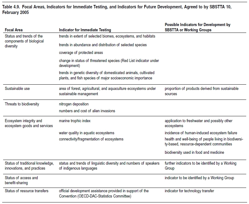
The first measures to move from the indicators for development to indicators for immediate testing seem likely to be the Red List Index (Butchart et al. 2004) and possibly also new measures of the extent and quality of key habitats. Coral reef extent may be assessed using established methods (Gardner et al. 2003), and there are likely to be other potential habitats whose extent can be assessed, using remote sensing techniques (such as mangroves).

4.5.2.2 Prospects for Meeting the 2010 Target

Despite the fact that at the time of writing there is no agreement on a complete set of indicators to be used for the 2010 target, various lines of evidence indicate that it is unlikely to be met. First, as evident from information in the preceding section, trends are still downwards for most species and populations, and the rate of decline is generally not slowing. The same is true also for data presented in aggregate indices such as the Living Planet Index (Loh and Wackermagel 2004), the Red List Index (Baillie et al. 2004), and the Pan-European Common Bird Monitoring Scheme (Gregory et al. 2003).

In the case of both the simple and aggregate measures, there are a few exceptions of species and ecosystems where declines are slowing or have been reversed. For example, the reduction in decline rates for some temperate woodland bird species and the recovery of some large mammals in Africa are testament to the potential success of effective management. These cases, however, generally result from management interventions that have been in place for many years and in some cases decades and they are in the minority.

For the species and [[habitat]s] that showed continuing decline in 2004, prospects for meeting the 2010 target will depend on sources of inertia and the time lag between a management intervention and the response. Natural sources of inertia correspond to the time scales inherent to natural systems; for example, all external factors being equal, population numbers grow or decline at a rate corresponding to the average turnover time or generation time. Even though meeting the 2010 target does not require recovery, many natural populations have generation times that limit the long-lasting improvements that can be realistically expected between now and 2010. On top of this is anthropogenic inertia resulting from the time scales inherent in human institutions for decision-making and implementation (MA 2003). For most systems these two sources of inertia will lead to delays of years, and more often decades, in slowing and reversing a declining biodiversity trend. This analysis assumes that the drivers of change could indeed be halted or reversed in the near term, although there is currently little evidence that any of the direct or indirect drivers are slowing or that any are well controlled at large to global scale.

The delay between a driver affecting a system and its consequences for biodiversity change can be highly variable. In the case of species extinctions this process has been well studied, and habitat loss appears to be one direct driver for which lag times will be long . In studies of African tropical forest bird species, the time from habitat fragmentation to species extinction has been estimated to have a half-life of approximately 50 years for fragments of roughly 1,000 hectares (Brooks et al. 1999). In Amazonian forest fragments of less than 100 hectares, half of the bird species were lost in less than 15 years, whereas fragments larger than 100 hectares lost species over time scales of a few decades to perhaps a century (Ferraz et al. 2003).

On the one hand, these time lags mean that estimates of current extinction rates may be underestimates of the ultimate legacy of habitat loss. For example, for African primate populations it is estimated that over 30% of species that will ultimately be lost as a result of historical deforestation still exist in local populations (Cowlishaw 1999). On the other hand, the time lags offer opportunities for interventions to be put in place to slow or reverse the trends, so long as in this case the period to habitat recovery is shorter than the time to extinction.

4.5.3 Key Gaps in Knowledge and Data

Certain gaps in knowledge and data relating to biodiversity are almost certain to prove critical over coming years, and efforts are urgently needed to gather this information, particularly if biodiversity indicators are to become more reliable and informative.

•  ?Data are sparse for certain key taxa—especially invertebrates, plants, fungi, and significant groups of microorganisms, including those in the soil. These groups are especially important for ecosystem services, yet global syntheses and trend information on even significant subsets are entirely missing. It seems likely that both extinction rates and local diversity and endemism may be lower among microorganisms than in the well-studied groups, suggesting that intense monitoring (Environmental monitoring and assessment) may not be so important. However this remains to be validated. Taxonomy as a discipline underpins much of this work yet is in decline worldwide.
•  ?Conservation assessment has proceeded at increased intensity over recent decades. However, knowledge of biodiversity trends falls far behind knowledge of status. Too often assessments are undertaken using new methods, new measures, or new places. Trends, which are critical to current questions, rely on a time series of comparable measures.
•  ?Local and regional datasets are generally of higher quality and cover longer time periods than global data. A better understanding of the relationship of local to global processes and the development of techniques to allow local dynamics to inform large-scale [[assessment]s] would allow rapid progress to be made in large to global-scale assessments.
•  ?There are far fewer studies at the genetic level than for populations, species, and ecosystems, yet these are significant components of biodiversity for assessing present and future adaptability to changing environments.
•  ?Marine and freshwater (Freshwater biomes) areas are less well known than terrestrial areas. Among terrestrial habitats, biodiversity trends in biomes such as drylands and [[grassland]s] are less well known than trends in forests.
•  ?The impacts of biodiversity change on ecosystems services are still poorly understood. Even where knowledge is better, there are almost no studies documenting the trends over time.

Alongside new data, approaches to long-term, large-scale continuous monitoring of biodiversity and attitudes to data sharing will need to be developed, as well as the infrastructure and technical and human resources that such an effort will require.

4.6 A Summary of Biodiversity Trends

The evidence presented in this chapter supports three broad conclusions about recent and impending changes in the amount and variability of biodiversity: there have been and will continue to be substantial changes that are largely negative and largely driven by people; these changes are varied—taxonomically, spatially, and temporally; and the changes are complex, in several respects.

First, changes are substantial and predominantly negative. Although there are very real limitations in the extent and quality of our knowledge of the changing state of nature, we already have overwhelming evidence that humans have caused the loss of a great deal of biodiversity over the past 50,000 years and that rates of loss have accelerated sharply over the past century. Current rates of species extinction are at least two orders of magnitude above background rates and are expected to rise to at least three orders above background rates.

Among extant species, 20% of all species in those groups that have been comprehensively assessed (mammals, birds, amphibians, conifers, and cycads) are believed to be threatened with extinction in the near future. For birds (the only taxon for which enough data are available), this proportion has increased since 1988 (BirdLife 2004a). Even among species not threatened with extinction, the past 20–40 years have seen substantial declines in population size or the extent of range in most groups monitored. These include European and North American farmland birds, large African mammals, nearly 700 vertebrate populations worldwide (Loh 2002), British birds, waders worldwide (IWSG et al. 2002), British butterflies and plants (Thomas et al. 2004a), amphibians worldwide (Houlahan et al. 2000; Alford and Pechmann 2001; Stuart et al. 2004), and most commercially exploited fish. These declines in populations are broadly mirrored by declines in the extent and condition of natural habitats (Jenkins et al. 2003).

Second, changes are varied. Rates of biodiversity decline, although very largely negative, vary widely on at least three dimensions. Taxonomically, certain groups appear more vulnerable to change than others: thus amphibians, and freshwater organisms in general, exhibit higher levels of threat and steeper rates of population decline than do better-known groups such as birds or mammals (Houlahan et al. 2000; Alford and Pechmann 2001; Loh 2002). Within groups, phylogenetically distinct, ancient, and species-poor lineages seem consistently to be faring disproportionately badly. Some generalist species are expanding their ranges, either naturally or as invasive aliens, whereas many ecological specialists are in decline.

Spatially, most species losses to date have been concentrated on islands. Disproportionately high rates of contemporary habitat conversion in endemic-rich areas of the tropics, where areas of dense human settlement and high species richness tend to coincide, mean that impending extinctions are particularly concentrated in tropical island and montane systems. In temperate regions, in contrast, substantial historical reductions in habitat extent have led to relatively few global extinctions (due in part to species having larger ranges at higher latitudes). Currently, populations and habitats are expanding in some temperate regions, such as temperate forests (Jenkins et al. 2003). Freshwater and marine patterns are less well documented.

Temporally, two patterns stand out. The first is that the scale of loss is in general increasing (although it is important to note that, both on land and at sea, preindustrial human-caused losses were also very substantial (Jackson 1994; Jackson et al. 2001)). The second pattern is that the anthropogenic drivers of loss are also changing; for example, invasive species and overexploitation were the predominant causes of bird extinctions in historic times, while habitat conversion, especially to agriculture, is the most significant driver currently facing threatened species (Baillie et al. 2004; BirdLife 2004a), with climate change predicted to emerge as another major threat in the near future (Thomas et al. 2004a).

Third, changes are complex. Besides variety, the overriding feature of biodiversity is its complexity. Patterns of biodiversity loss are in turn correspondingly complex, in several respects. Species, populations, and ecosystems differ not just in their exposure but also in their vulnerability to anthropogenic drivers of change. In addition, complex interactions within communities mean that changes in the abundance of one species will often have broad-ranging effects through a system. (See also Chapter 12.) One well-documented example is the recent switch by Aleutian island killer whales to hunting sea otters instead of pinnipeds (likely triggered by fishing-related declines in pinnipeds); this has greatly reduced sea otter numbers, allowing the population and grazing pressure of sea urchins to increase, in turn leading to a dramatic decline in kelp density (Estes et al. 1998). In Australia, the deliberate introduction of African grasses (such as gamba grass, Andropogon gayanus) to native woody savannas has also increased the intensity of frequent, very intense fires due to the highly flammable nature of the introduced grasses (Rossiter et al. 2003); as elsewhere (D’Antonio and Vitousek 1992), changes in the fire regime in turn reduced native tree and shrub cover, thereby accelerating the invasion of fire-tolerant aliens and resulting in a wholesale ecosystem shift from woody vegetation to open grassland.

Another aspect of the complexity is that community dynamics mean threats themselves rarely operate in isolation (Myers 1995). The impact of climate change, for example, is predicted to be far more marked where habitat transformation and fragmentation blocks the movement of species in response to shifting climate (Thomas et al. 2004a), a hypothesis recently supported by data on U.K. butterflies (Warren et al. 2001). Similarly, there is now growing evidence of synergistic effects of increased UV-B exposure, acidification, and pathogens on declining amphibian populations (Kiesecker and Blaustein 1995; Long et al. 1995) and of synergistic effects between logging, forest fragmentation, and fire in tropical forests (Cochrane et al. 1999; Cochrane 2003).

It is also becoming clear that often ecosystems respond not linearly to external changes but in a stepwise manner (Myers 1995). Thus cumulative biotic or abiotic pressures that at first appear to have little effect may lead to quite sudden and unpredictable changes once thresholds are crossed (Scheffer et al. 2001). Moreover, such thresholds may become lower as anthropogenic impacts simplify systems and reduce their intrinsic resilience to change. (See also Chapter 12.) One well-studied example is the sudden switch in 1983 from coral to algal domination of Jamaican reef systems. This followed several centuries of overfishing of herbivores (Herbivory), which left the control of algal cover almost entirely dependent on a single species of sea urchin, whose populations collapsed when exposed to a species-specific pathogen (Hughes 1994; Jackson 1997). As a result, Jamaica’s reefs shifted (apparently irreversibly) to a new low diversity, algal-dominated state with very limited capacity to support fisheries (Fisheries and aquaculture) (McManus et al. 2000). Given their potential importance, much more work is needed on whether threshold effects such as this are typical, how reversible they are, and where thresholds lie.

Extrapolation from current trends suggests that both the amount and variability of nature will continue to decline over much of Earth (UNEP 2002a; Jenkins et al. 2003). The exception is likely to be in some industrial countries, where forest cover may continue to increase and, with it, the population sizes of many forest-dependent species. In contrast, clearance of natural [[habitat]s], reductions of populations, and the associated loss of populations and indeed species look set to persist and even accelerate across much of the tropics and across many if not most aquatic systems. Particularly vulnerable areas include cloud forests, coral reefs, mangroves (threatened by the synergistic effects of climate change and habitat clearance), all but the very largest blocks of tropical forest, and most freshwater (Freshwater biomes) habitats. Particularly vulnerable taxa include large marine species, large-bodied tropical vertebrates, and many freshwater groups (Jenkins et al. 2003).

References

• Agapow, P.-M., O.R.P. Bininda-Emonds, K.A. Crandall, J.L. Gittleman, G.M. Mace, J.C. Marshall, and A. Purvis, 2004: The impact of species concept on biodiversity studies. Quarterly Review of Biology, 79, 161–179.
• Alford, R.A. P.M. Dixon and J.H.K. Pechmann, 2001: Global Amphibian population declines. Nature, 412, 499–500.
• Alroy, J., 1998: Equilibrial diversity dynamics in North American mammals. In: Biodiversity dynamics, turnover of populations, taxa, and communities, M.L. McKinney and J.A. Drake (eds.), Columbia University Press, New York, 232–287.
• Alroy, J., 2001: A multi-species overkill simulation of the end-Pleistocene megafaunal mass extinction. Science, 292, 1893–1986.
• Anderson, S., 1994: Area and endemism. Quarterly Review of Biology, 69, 451– 471.
• Anstey, S., 1991: Wildlife Utilisation in Liberia (World Wide Fund for Nature and FDA Wildlife Survey). World Wide Fund for Nature and FDA, Gland, Switzerland.
• APG (Angiosperm Phylogeny Group), 1998: An ordinal classification for the families of flowering plants. Annals of the Missouri Botanic Garden, 85, 531– 553.
• Atkinson, A.I.E., 1985: The spread of commensal species of Rattus to oceanic islands and their effects on island avifaunas. In: The Conservation of Island Birds. Case Studies for the Management of Threatened Bird Species, P.J. Moors (ed.), ICBP, Cambridge.
• Atkinson, C.T., R.J. Dusek, K.L. Woods, and W.M. Iko, 2000: Pathogenicity of avian malaria in experimentally-infected Hawaii Amakihi. Journal of Wildlife Diseases, 36(2), 197–204.
• Atkinson, I.A.E. and E.K. Cameron, 1993: Human Influence On the Terrestrial Biota and Biotic Communities of New-Zealand. Trends in Ecology & Evolution, 8(12), 447–451.
• Avise, J.C. and G.C. Johns, 1999: Proposal for a standardized temporal scheme of biological classification for extant species. Proceedings of the National Academy of Science USA, 96, 7358–7363.
• Bailey, R.G., 1989: Explanatory supplement to Ecoregions map of the continents. Environmental Conservation, 16, 307–309.
• Bailey, R.G., 1998: Ecoregions: the ecosystem geography of oceans and continents. Springer-Verlag, New York.
• Bailey, R.G. and H.C. Hogg, 1986: A world ecoregions map for resource partitioning. Environmental Conservation, 13, 195–202.
• Baillie, J.E.M., C. Hilton-Taylor, and S.N. Stuart, 2004: 2004 IUCN Red List of Threatened Species. A Global Species Assessment. IUCN, Gland, Switzerland.
• Balcalbaca-Dobrovici, N., 1989: The Danube River and it’s Fisheries. In: Proceedings of the International Large River Symposium, D.P. Dodge (ed.). 106, 455–468.
• Balmford, A., 1996: Extinction filters and current resilience: the significance of past selection pressures for conservation biology. Trends in Ecology & Evolution, 11(5), 193–196.
• Balmford, A., 1999: (Less and less) great expectations. Oryx, 33, 87–88.
• Balmford, A. and A. Long, 1994: Avian endemism and forest loss. Nature, 372, 623–624.
• Balmford, A., M.J.B. Green, and M.G. Murray, 1996: Using higher-taxon richness as a surrogate for species-richness: I. Regional tests. Proceedings of the Royal Society of London, series B Biological Sciences, 263, 1267–1274.
• Balmford, A., R.E. Green, and M. Jenkins, 2003a: Measuring the changing state of nature. Trends in Ecology & Evolution, 18(7), 326–330.
• Balmford, A., K.J. Gaston, S. Blyth, A. James, and V. Kapos, 2003b: Global variation in terrestrial conservation costs, conservation benefits, and unmet conservation needs. Proceedings of the National Academy of Sciences of the United States of America, 100(3), 1046–1050.
• Balmford, A., P. Crane, A. Dobson, R.E. Green, and G.M. Mace, 2005: The 2010 challenge: data availability, information needs, and extraterrestrial insights. Philosophical Transactions of the Royal Society of London B. 360:221–228.
• Barnes, R.F.W., G.C. Craig, H.T. Dublin, G. Overton, W. Simmons, and C.R. Thouless, 1999: African Elephant Database 1998. IUCN, Gland, Switzerland.
• Barrett, S.C., 1989: Water Weed Invasions. Scientific American, October, 90–97.
• Barthlott, W., N. Biedinger, G. Braun, F. Feig, G. Kier, and J. Mutke, 1999: Terminological and methodological aspects of the mapping and analysis of global biodiversity. Acta Botanica Fennica, 162, 103–110.
• Baum, J.K., R.A. Myers, D.G. Kehler, B. Worm, S.J. Harley, and P.A. Doherty, 2003: Collapse and conservation of shark populations in the Northwest Atlantic. Science, 299(5605), 389–392.
• Bawa, K.S. and S. Dayanandan, 1997: Socioeconomic factors and tropical deforestation. Nature, 386, 562–563.
• Bennett, E.L., A. Nyaoi, and J. Sompud, 2000: Saving Borneo’s Bacon: The Sustainability of Hunting in Sarawak and Sabah. In: Hunting for Sustainability, J.G. Robinson and E.L. Bennett (eds.), Columbia Press, New York, 305– 324.
• Bennett, P.M. and I.P.F. Owens, 1997: Variation in extinction risk among birds: Chance or evolutionary predisposition? Proceedings of the Royal Society of London Series B-Biological Sciences, 264(401–408).
• Berger, L., R. Speare, P. Daszak, D.E. Green, A.A. Cunningham, et al. 1998: Chytridiomycosis causes amphibian mortality associated with population declines in the rainforests of Australia and Central America. Proceedings of the National Academy of Sciences of the United States of America, 95, 9031–9036.
• Berra, T.M., 2001: Freshwater fish distribution. Academic Press, San Diego.
• BirdLife, 2004a: Threatened Birds of theWorld 2004. Birdlife International, Cambridge, UK.
• BirdLife, 2004b: State of the World’s Birds 2004—Indicators for our changing world. BirdLife International, Cambridge, U.K.
• Bisby, F.A., 1995: Characterization of biodiversity. In: Global Biodiversity Assessment, V.H. Heywood (ed.), Cambridge University Press, Cambridge.
• Bisby, F.A., J. Shimura, M. Ruggiero, J. Edwards, and C. Haeuser, 2002: Taxonomy, at the click of a mouse. Nature, 418, 367.
• Bogan, A.E., 1997: The Silent Extinction. American Paleontologist, 5(1), 2–4.
• Boulinier, T., J.D. Nichols, J.E. Hines, J.R. Sauer, C.H. Flather, and K.H. Pollock, 2001: Forest fragmentation and bird community dynamics: Inference at regional scales. Ecology, 82(4), 1159–1169.
• Bramwell, D., 2002: How many plant species are there? Plant Talk, 28, 32–33.
• Briggs, J., 1974: Marine Zoogeography. McGraw-Hill, New York.
• Brook, B.W. and D. Bowman, 2004: The uncertain blitzkrieg of Pleistocene megafauna. Journal of Biogeography, 31, 517–523.
• Brooks, T.M., S.L. Pimm, and J.O. Oyugi, 1999: Time lag between deforestation and bird extinction in tropical forest fragments. Conservation Biology, 13, 1140–1150.
• Brown, B.E., R.P. Dunne, M.S. Goodson, and A.E. Douglas, 2000: Bleaching patterns in coral reefs. Nature, 404, 142–143.
• Brown, J.H., 1984: On the relationship between abundance and distribution of species. American Naturalist, 124, 255–279.
• Butchart, S.H.M., A.J. Stattersfield, L.A. Bennun, S.M. Shutes, H.R. Ackakaya, et al. 2004: Measuring global trends in the status of biodiversity: Red List Indices for Birds. PLoS. Biology, 2(12), e383.
• Butchart, S.H.M., A.J. Stattersfield, J. Baillie, L.A. Bennun, S.N. Stuart, et al. 2005, Using Red List Indices to measure progress towards the 2010 target and beyond. Philosophical Transactions of the Royal Society. Series B., 360, 255–268.
• Castro, J.I., C.M. Woodley, and R.L. Brudek, 1999: A preliminary evaluation of the status of shark species (FAO Fisheries Technical Paper no. 380). FAO (Fisheries), Rome.
• Ceballos, G. and P.R. Ehrlich, 2002: Mammal population losses and the extinction crisis. Science, 296, 904–907.
• Channell, R. and M.V. Lomolino, 2000: Dynamic biogeography and the conservation of endangered species. Nature, 403, 84–86.
• Chape, S., S. Blyth, L. Fish, P. Fox, and M. Spalding, 2003: 2003 United Nations List of Protected Areas. I.a. UNEP (ed.)Gland, Switzerland.
• Cheke, A.S., 1987: An ecological history of the Mascarene Islands, with particular reference to extinctions and introductions of land vertebrates. In: Studies of Mascarine Island birds, A.W. Diamond (ed.), Cambridge University Press, Cambridge, 5–89.
• Claridge, M.F., H.A. Dawah, and M.R. Wilson, 1997: Species: The Units of Biodiversity. Chapman & Hall, London.
• Cochrane, M.A., 2003: Fire science for rainforests. Nature, 421(6926), 913– 919.
• Cochrane, M.A., A. Alencar, M.D. Schulze, C.M. Souza, D.C. Nepstad, P. Lefebvre, and E.A. Davidson, 1999: Positive feedbacks in the fire dynamic of closed canopy tropical forests. Science, 284(5421), 1832–1835.
• Colwell, R.K. and D.C. Lees, 2000: The mid-domain effect: geometric constraints on the geography of species richness. Trends in Ecology and Evolution, 15, 70–76.
• Cowlishaw, G., 1999: Predicting the Pattern of Decline of African Primate Diversity: an Extinction Debt from Historical Deforestation. Conservation Biology, 13, 1183–1193.
• Cracraft, J., 1983: Species concepts and speciation analysis. Current Ornithology, 1, 159–187.
• Crandall, K.A., O.R.P. Bininda-Emonds, G.M. Mace, and R.K.Wayne, 2000: Considering evolutionary processes in conservation biology. Trends in Ecology & Evolution, 15(7), 290–295.
• Crooks, K.R. and M.E. Soule, 1999: Mesopredator release and avifaunal extinctions in a fragmented system. Nature, 400(6744), 563–566.
• Cumming, D.H.M., R.F. du Toit, and S.N. Stuart, 1990: African Elephants and Rhinos. Status Survey and Conservation Action Plan., IUCN, Gland, Switzerland.
• Curtis, T.P., W.T. Sloan, and J.W. Scannell, 2002: Estimating prokaryotic diversity and its limits. Proceedings of the National Academy of Sciences of the United States of America, 99(16), 10494–10499.
• D’Antonio, C.M. and P.M. Vitousek, 1992: Biological invasions by exotic grasses, the grass-fire cycle, and global change. Annual Review of Ecology and Systemantics, 23, 63–87.
• Darwall, W. and C. Revenga ((in prep)): Inland Water Ecosystems. In The State of the Worlds Protected Areas. IUCN, Gland, Switzerland and Cambridge.
• Daszak, P., A.A. Cunningham, and A.D. Hyatt, 2000: Emerging Diseases of Wildlife—Threats to Biodiversity and Human Health. Science, 287(443–449).
• Daszak, P., A.A. Cunningham, and A.D. Hyatt, 2001: Anthropogenic environmental change and the emergence of infectious diseases in wildlife. Acta Tropica, 78, 103–116.
• De Meulenaer, T. and C. Raymakers, 1996: Sturgeons of the Caspian Sea and the International Trade in Caviar., TRAFFIC, TRAFFIC Europe., Brussels, Belgium.
• Dekker, W., 2003: Eel stocks dangerously close to collapse., ICES (International Council for the Exploration of the Sea), Copenhagen, Denmark.
• Delany, S.N., C. Reyes, E. Hubert, S. Pihl, E. Rees, L. Haanstra, and A. van Strien, 1999.: Results from the International Waterbird Census in the Western Palearctic and Southwest Asia, 1995 and 1996. 54, Wetlands International Publication No. 54., Wageningen, The Netherlands:.
• Diamond, J.M., 1972: Biogeographic kinetics: estimation of relaxation times for avifaunas of Southwest Pacific Islands. Proceedings of the National Academy of Sciences, USA, 69, 3199–3203.
• Dietrich, G., 1963: General Oceanography: An Introduction. John Wiley, New York.
• Dirzo, R. and P.H. Raven, 2003: Global state biodiversity and loss. Annual Review of Environmental Resources, 28, 137–167. Dobson, A. and J. Foufopoulos, 2001: Emerging infectious pathogens of wildlife. Philosophical Transactions of the Royal Society of London B, 356, 1001.
• Dobzhansky, T., 1950: Mendelian populations and their evolution. American Naturalist, 84, 401–418.
• Doubleday, W.G., 2001: Is Atlantic Salmon Aquaculture a Threat to Wild Stocks in Altantic Canada? ISUMA: Canadian Journal of Policy Research 2, 2(1).
• Dulvy, N.K., Y. Sadovy, and J.D. Reynolds, 2003: Extinction vulnerability in marine populations. Fish and Fisheries, 4, 25–64.
• Dynesius, M.a.C.N., 1994: Fragmentation and Flow Regulation of River Systems in the Northern Third of the World. Science, 266, 753–762.
• East, R., 1999: African Antelope Database 1998. IUCN, Gland, Switzerland.
• Easterling, W.E., J.R. Brandle, C.J. Hays, Q. Guo, and D.S. Guertin, 2001: Simulating the impact of human land use change on forest composition in the Great Plains agroecosystems with the Seedscape model. Ecological Modelling, 140, 163–176.
• Ehrlich, P.R., 1994: Energy use and biodiversity loss. Philosophical Transactions of the Royal Society of London B: Biological Sciences, 344, 99–104.
• Emslie, R. and M. Brooks, 1999: African Rhino. Stauts Survey and Conservation Action Plan. IUCN, Gland, Switzerland.
• Environment Canada and U.S. EPA (Environmental Protection Agency), 2003: Great Lakes Atlas. Living Resources. Environment Canada and U.S. EPA. Ottawa, Canada.
• Erwin, T.L., 1982: Tropical forests: their richness in Coleoptera and other Arthropod species. The Coleopterist’s Bulletin, 36, 74–75.
• Estes, J.A., M.T. Tinker, T.M. Williams, and D.F. Doak, 1998: Killer Whale Predatoin on Sea Otters Linking Oceanic and Nearshore Ecosystems. Science, 282, 473–476.
• European Council, 2001: Presidency Conclusions. SN/200/1/01 REV1, Goteburg Council.
• Everett, R.A., 2000: Patterns and pathways of biological invasions. Trends in Ecology & Evolution, 15, 177–178.
• Faith, D.P., 1992: Conservation evaluation and phylogenetic diversity. Biological Conservation, 61, 1–10.
• FAO (Food and Agriculture Organization of the United Nations), 1997: The State of the World’s Forests 1997. Rome, Italy.
• FAO, 1999: Review of the State of World Fishery Resources: Inland Fisheries. FAO Inland Water Resources and Aquaculture Service, Fishery Resources Division. FAO Fisheries Circular No. 942, Rome.
• FAO, 2000a: The State of theWorld’s Fisheries and Aquaculture 2000. FAO, Rome.
• FAO, 2000b: Global Forest Resource Assessment 2000. Food and Agriculture Organization, Rome.
• FAO, 2001a: Global Forest Resources Assessment 2000 Main Report. FAO Forest Paper 140, Food and Agriculture Organization of the United Nations, Rome, 479 pp.
• FAO, 2001b: Forest Resources Assessment 2000. FAO Forestry Paper 140, FAO, Rome.
• FAO, 2002: State of the World’s Fisheries and Aquaculture Report 2002. FAO.
• FAO, 2003: State of the World’s Forest 2003. FAO, Rome.
• Fekete, B., C.J. Vörösmarty, and W. Grabs, 1999: Global, Composite Runoff Fields Based on Observed River Discharge and Simulated Water Balance. World Meteorological Organization Global Runoff Data Center Report No. 22., Koblenz, Germany.
• Ferraz, G., G.J. Russell, P.C. Stouffer, R.O. Bierregaard, S.L. Pimm, and T.E. Lovejoy, 2003: Rates of species loss from Amazonian forest fragments. Procedings of the National Academy of Sciences of the USA, 100(24), 14069–14073.
• Finlay, B.F. and T. Fenchel, 2004: Cosmopolitan Metapopulations of Free- Living Microbial Eukaryotes. Protist, 155, 237–244.
• Finlayson, C. M., G. W. Begg, J. Howes, J. Davies, K. Tagi, and L. Lowry, 2002. Asian Wetland Inventory, Wetlands International, Netherlands.
• Fisher, D.O., S.P. Blomberg, and I.P.F. Owens, 2003: Extrinsic versus intrinsic factors in the decline and extinction of Australian marsupials. Proceedings of the Royal Society of London Series B-Biological Sciences, 270, 1801–1808.
• Fitter, A.H., 2005. Darkness visible: reflections on underground ecology. Journal of Ecology, 93, 231–243.
• FitzGibbon, C.D., H. Mogaka, and J. Fanshawe, 2000: Threatened Mammals, Subsistence Harvesting, and High Human Population Densities: A recipe for disaster? In: Hunting for Sustainability, J.G. Robinson and E.L. Bennett (eds.), Columbia Press, New York, 154–167.
• Fjeldså, J. and C. Rahbek, 1998: Continent-wide conservation priorities and diversification processes. In: Conservation in a changing world, G.M. Mace, A. Balmford, and J.R. Ginsberg (eds.), Cambridge University Press, Cambridge, UK, 139–160.
• Foose, T.J. and N. van Strien, 1997: Asian Rhinos. Status Survey and Conservation Action Plan (2nd Edition). IUCN, Gland, Switzerland.
• Foote, M., 1997: Estimating taxonomic durations and preservation probability. Palaeobiology, 23, 278–300.
• Ford, R.G., 1999: Defining Marine Ecoregions of the Pacific Continental United States. In: Terrestrial ecoregions of North America: a conservation assessment., T.e.a. Ricketts (ed.), Island Press, Washington DC.
• Frankham, R., 1995: Conservation genetics. Annual Review Genetics, 29, 305– 327.
• Frankham, R., B.J. D., and D.A. Briscoe, 2002: Introduction to Conservation Genetics. Cambridge University Press, Cambridge, UK.
• Freitag, S., A.O. Nicholls, and A.S. van Jaarsveld, 1998: Dealing with established reserve networks and incomplete distribution data sets in conservation planning. South African Journal of Science, 94, 79–86.
• Fritts, T.H. and G.H. Rodda, 1998: The role of introduced species in the degradation of island ecosystems: A case history of Guam. Annual Review of Ecology and Systematics, 29, 113–140.
• Froese, R. and D.E. Pauly, 2003: FishBase.World Wide Web electronic publication. [Internet] Cited 12 November 2003. Available at www.fishbase.org.
• Gardner, T.A., I.M. Cote, J.A. Gill, A. Grant, and A.R. Watkinson, 2003: Long-term region-wide declines in Caribbean corals. Science, 301, 958–960.
• Gaston, K.J., 1991: The magnitude of global insect species richness. Conservation Biology, 5, 283–296.
• Gaston, K.J., 1994: Rarity. Chapman and Hall, London.
• Gaston, K.J., 1994a: Spatial patterns of species distribution: how is our knowledge of the global insect fauna growing? Biological Conservation, 67, 37–40.
• Gaston, K.J., 1996: Species-range-size distributions: patterns, mechanisms and implications. Trends in Ecology and Evolution, 11, 197–201.
• Gaston, K.J., 1998: Species-range size distributions: products of speciation, extinction and transformation. Philosophical Transactions of the Royal Society of London B, 353, 219–230.
• Gaston, K.J., 2000: Global patterns in biodiversity. Nature, 405, 220–227.
• Gaston, K.J. and R.M. May, 1992: Taxonomy of taxonomists. Nature, 356, 281–282.
• Gaston, K.J. and T.M. Blackburn, 1997b: Evolutionary age and risk of extinction in the global avifauna. Evolutionary Ecology, 11, 557–565.
• Gaston, K. J., Jones, A. G., Hänel, C. & Chown, S. L. 2003 Rates of species introduction to a remote oceanic island. Proceedings of the Royal Society of London Series B-Biological Sciences 270, 1091–1098.
• Gibbins, J.W., D.E. Scott, T.J. Ryan, K.A. Buhlmann, T.D. Tuberville, et al. 2000: The global decline of reptiles, déjà vu amphibians. BioScience, 50, 653–666.
• Gilpin, M.E. and M.E. Soulé, 1986: Minimum viable populations: processes of species extinctions. In: Conservation Biology—the Science of Scarcity and Diversity, M.E. Soule (ed.), Sinauer Associates, Michigan, 19–34.
• Godfray, H.C.J., 2002: Challenges for taxonomy: the discipline will have to reinvent itself if it is to flourish. Nature, 417, 17–19.
• Godfray, H.C.J., O.T. Lewis, and J. Memmott, 1999: Studying insect diversity in the tropics. Philosophical Transactions of the Royal Society of London B, 354, 1811–1824.
• Goldburg, R.J., M.S. Elliott, and R.L. Naylor, 2001: Marine Aquaculture in the United States: Environmental Impacts and Policy Options. Pew Oceans Commission. Arlington, Virgina.
• G?mez de Silva Garza, H., 1996: The conservation importance of semiendemic species. Conservation Biology, 10, 674–675.
• Goodman, D., 1987: The demography of chance extinction. In: Viable populations for conservation, M.E. Soule (ed.), Cambridge University Press, Cambridge, 11–34.
• Goodman, S.M. and B.D. Patterson (eds.), 1997: Natural change and Human Impact in Madagascar. Smithsonian Institution, Chicago.
• Govaerts, R., 2001: How many species of seed plants are there? Taxon, 50, 1085–1090.
• Grassle, J.F. and N.J. Maciolek, 1992: Deep-sea species richness: regional and local diversity estimates from quantitative bottom samples. American Naturalist, 139, 313–341.
• Green, R.E., A. Balmford, P.R. Crane, G.M. Mace, J.R. Reynolds, and R.K. Turner, 2005: Responding to the Johannesburg Challenge: A Framework for Improved Monitoring of Biodiversity. Conservation Biology 19, 56–65.
• Gregory, R.D., P. Vorisek, A.J. van Strien, M. Eaton, and S.R. Wotton, 2003: From bird monitoring to policy-relevant indicators. A report to the European Topic Centre on Nature Protection and Biodiversity.
• Griffiths, R.W., 1993: The changing environment of Lake St. Clair. Paper presented at the Third International Zebra Mussel Conference, Toronto, Canada.
• Groombridge, B. and M.D. Jenkins, 2002: World Atlas of Biodiversity. University of California Press, Berkeley.
• Hall, B.L. and R.E. Moreau, 1962: A study of the rare birds of Africa. Bulletin of the British Museum (Natural History) Zoology, 8, 313–378.
• Hammond, P.M., 1992: Species inventory. In: Global Biodiversity, B. Groombridge (ed.), Chapman & Hall, London, UK, 17–39.
• Harcourt, A.H., S.A. Parks, and R. Woodroffe, 2001: Human density as an influence on species/area relationships: double jeopardy for small African reserves? Biodiversity and Conservation, 10, 1011–1026.
• Harrison, I.J. and M.J. Stiassny, 1999: The Quiet Crisis: A Preliminary Listing of the Freshwater Fishes of the World that Are Extinct or ‘‘Missing in Action.’’ In: Extinctions in Near Time, MacPhee (ed.), New York: Kluwer Academic/ Plenum Publishers, New York, 271–331.
• Hawksworth, D.L., 1991: The fungal dimension of biodiversity: magnitude, significance and conservation. Mycological Research, 95, 641–655.
• Hayden, B., G. Ray, and R. Dolan, 1984: Classification of coastal and marine environments. Environmental Management, 11, 199–207.
• He, F. and K.J. Gaston, 2000: Estimating species abundance from occurrence. American Naturalist, 156, 553–559.
• Hebert, P.D.N., A. Cywinska, S.L. Ball, and J.R. De Waard, 2003: Biological identification through DNA barcodes. Proceedings of the Royal Society of London, series B Biological Sciences, 270, 313–321.
• Hedrick, P.W. and T.J. Kim, 2000: Genetics of complex polymorphisms: parasites and maintenance of MHXC variation. In: Evolutionary Genetics from Molecules to Morphology, R.S.S.C.K. Krimbas (ed.), Cambridge University Press, Cambridge, UK, 204–234.
• Hey, J., 2001: The mind of the species problem. Trends in Ecology and Evolution, 16, 326–329.
• Heywood, V.H. and R.T. Watson (eds.), 1995: Global Biodiversity Assessment. United Nations Environment Programme., Cambridge, U.K.
• Hill, G., J.Waage, and G. Phiri, 1997: TheWater Hyacinth Problem in Tropical Africa. In: Proceedings of the International Water Hyacinth Consortium, e. E.S. Delfosse and N.R. Spencer (ed.) Washington, DC:.
• Hill, J.K., C.D. Thomas, and B. Huntley, 1999: Climate and habitat availability determine 20th century changes in a butterfly’s range margin. Proceedings of the Royal Society of London B, 266, 1197–1206.
• Hillebrand, H., 2004: Strength, slope and variability of marine latitudinal gradients. Marine Ecology-Progress Series, 273, 251–267.
• Hilton-Taylor, C.C., 2000: 2000 IUCN Red List of Threatened Species. IUCN, Gland, Switzerland and Cambridge, UK, 61 pp.
• Hodgson, G. and J. Liebeler, 2002: The Global Coral Reef Crisis: Trends and Solutions. Reef Check Foundation, Los Angeles.
• Hodkinson, I.D., 1992: Global insect diversity revisited. Journal of Tropical Ecology, 8, 505–508.
• Hodkinson, I.D. and D. Casson, 1991: A lesser predilection for bugs: Hemiptera (Insecta) diversity in tropical rain forests. Biological Journal of the Linnean Society, 43, 101–109.
• Hoenig, J.M. and S.H. Gruber, 1990: Life-history patterns in the elasmobranches: implications for fisheries management. In: Elasmobranchs as Living Resources: Advances in the Biology, Ecology, Systematics, and the Status of Fisheries. Technical Report NMFS 90, H.L. Pratt Jr., S.H. Gruber, and T. Taniuchi (eds.), US Department of Commerce National Oceanic and Atmospheric Administration (NOAA), 1–16.
• Houlahan, J.E., C.S. Findlay, B.R. Schmidt, A.H. Meyer, and S.L. Kuzmin, 2000: Quantitative evidence for global amphibian population declines. Nature, 404, 752–755.
• Hughes, J.B., G.C. Daily, and P.R. Ehrlich, 1997: Population diversity: its extent and extinction. Science, 278, 689–692.
• Hughes, T.P., 1994: Catastrophes, phase shifts, and large-scale degradation of a Caribbean coral reef. Science, 265, 1547–1551.
• Hughes, T.P., A.H. Baird, D.R. Bellwood, M. Card, S.R. Connolly, et al. 2003: Climate Change, Human Impacts, and the Resilience of Coral Reefs. Science, 301, 929–933.
• Hull, D.L., 1997: The ideal species concept -and why we can’t get it. In: Species: The Units of Biodiversity, M.F. Claridge, H.A. Dawah, and M.R. Wilson (eds.), Chapman and Hall, London, 357–380.
• Huntley, B. and T. Webb, 1989: Migration: species’ response to climatic variations caused by changes in the earth’s orbit. Journal of Biogeography, 16, 5–19.
• Huntsman, G.R., J. Potts, R.W. Mays, and D. Vaughan, 1999: Groupers (Serranidae, Epinephelinae): endangered apex predators of reef communities. In: Life in the Slow Lane: ecology and Conservation of Long-lived Marine Animals. Symposium 23, J.A. Musick (ed.), American Fisheries Society, Bethesda, MD, USA, 217–231.
• Hutchings, J.A., 2000: Collapse and recovery of marine fishes. Nature, 406, 882–885.
• Hutchings, J.A. and J.D. Reynolds, 2004: Marine fish stock population collapses: consequences for recovery and extinction risk. BioScience, 54, 297– 309.
• IIED (International Institute for Environment and Development) and Traffic, 2002: Making a Killing or Making a Living: Wildlife trade, trade controls and rural livelihoods. London, UK.
• Imhoff, M.L., L. Bounoua, T.H. Ricketts, C. Loucks, A.H. Harris, and W.T. Lawrence, 2004: Human Consumption of Net Primary Production. Nature. 429, 870–3.
• Imhoff, M.L., L. Bounoua, T.H. Ricketts, C. Loucks, R. Harriss, and W.T. Lawrence, in review: The geography of consumption: Human appropriation of NPP.
• Isaac, N.J.B., J. Mallett, and G.M. Mace, 2004: Taxonomic inflation: its influence on macroecology and conservation. Trends in Ecology and Evolution, 19(9), 464–469.
• IUCN (World Conservation Union), 2001: IUCN Red List Categories and Criteria. Version 3.1. IUCN, Gland, Switzerland.
• IUCN, 1994: Guidelines for Protected Area Management Categories, IUCN Commission on National Parks/World Conservation Monitoring Centre, The World Conservation Union, Gland, Switzerland
• Iverson, J.B., A.R. Kiester, L.E. Hughes, and A.J. Kimerling, 2003: The EMY System World Turtle Database 2003. Oregon State University. Available at http://emys.geo.orst.edu.
• IWSG (International Wader Study Group) D.A. Stroud, N.C. Davidson, R. West, D.A. Scott, L. Haanstra, O. Thorup, B. Ganter, and S. Delany (compilers), 2002: Status of migratory wader populations in Africa and Western Eurasia in the 1990s. 15, International Wader Studies 15.
• Jablonski, D., 1986: Background and mass extinctions: the alternation of macroevolutionary regimes. Science, 231, 129–133.
• Jackson, J.B.C., 1994: Constancy and change of life in the sea. Philosophical Transactions of the Royal Society Series B, 344, 55–60.
• Jackson, J.B.C., 1997: Reefs since Columbus. Coral Reefs, 16, Suppl.: S23— S32.
• Jackson, J.B.C., 2001: What was natural in the coastal oceans? Proceedings of the National Academy of Sciences, USA, 98, 5411–5418.
• Jackson, J.B.C., M.X. Kirby, W.H. Berger, K.A. Bjorndal, L.W. Botsford, et al., 2001: Historical Overfishing and the Recent Collapse of Coastal Ecosystems. Science, 293, 629–637.
• Jenkins, R.K.B., L.D. Brady, M. Bisoa, J. Rabearivony, and R.A. Griffiths, 2003: Forest disturbance and river proximity influence chameleon abundance in Madagascar. Biological Conservation, 109(3), 407–415.
• Karg, J. and L. Ryszkowski, 1996: Animals in arable land. In: Dynamics of an agricultural landscape, L. Ryszkowski, French N. and Kedziora A (ed.), Panstwowe Wydawnictwo Rolnicze i Lesne, Poznan, 138–172.
• Karr, J.R. and D.R. Dudley, 1981: Index of Biotic Integrity for Aquatic Systems. Environmental Management., 5, 44–68.
• Khan, M.b.M.K., 1989: Asian Rhinos. An Action Plan for their Conservation. IUCN, Gland, Switzerland.
• Kier, G., J. Mutke, W. Kueper, H. Kreft, and W. Barthlott, 2002: Richness of vascular plant species of the terrestrial ecoregions of the world. Unpublished report, University of Bonn Botanical Institute, Bonn, 2002.
• Kiesecker, J.M. and A.R. Blaustein, 1995: Synergism between Uv-B Radiation and a Pathogen Magnifies Amphibian Embryo Mortality in Nature. Proceedings of the National Academy of Sciences of the United States of America, 92(24), 11049–11052.
• Klein Goldewijk, K., 2001: Estimating global land use change over the past 300 years: the HYDE database. Global Biogeochemical Cycles, 15, 417–434.
• Koh, L.P., R.R. Dunn, N.S. Sodhi, R.K. Colwell, H.C. Proctor, and V.S. Smith, 2004: Species coextinctions and the biodiversity crisis. Science, 305(5690), 1632–1634.
• Kura, Y., C. Revenga, E. Hoshino, and G. Mock, 2004: Fishing for Answers: Making Sense of the Global Fish Crisis, World Resources Institute,Washington, DC.
• Lande, R., 1993: Risks of Population Extinction from Demographic and Environmental Stochasticity and Random Catastrophes. American Naturalist, 142 (- 6), 911–927.
• Laurance, W.F., M.A. Cochrane, S. Bergen, P.M. Fearnside, P. Delamonica, C. Barber, S. D’Angelo, and T. Fernandes, 2001: The future of the Brazilian Amazon. Science, 291, 438–439.
• Laurance, W.F., R.O. Bierregaard Jr., C. Gascon, R.K. Didham, A.P. Smith, et al. 1997: Tropical forest fragmentation: synthesis of a diverse and dynamic discipline. In: Tropical Forest Fragments, W.F. Laurance and R.O. Bierregaard (eds.), University of Chicago Press, 502–514.
• Lavelle, P. and E. Lapied, 2003: Endangered earthworms of Amazonia: an homage to Gilberto Righi. Pedobiologia, 47(5–6), 419–427.
• Lelek, A., 1989: The Rhine River and Some of it’s Tributaries Under Human Impact in the Last Two Centuries. In: Proceedings of the International Large River Symposium., D.P. Dodge (ed.). 106, 469–487.
• Lévêque, C., 1997.: Biodiversity dynamics and conservation: the freshwater fish of tropical Africa. Cambridge University Press., Cambridge, UK.
• Levine, J.M., 2000: Species-diversity and biological invasions: relating localprocess to community pattern. Science, 288, 852–854.
• Liao, G.Z., K.X. Lu, and X.Z. Xiao, 1989: Fisheries Resources of the Pearl River and their Exploitation. In: Proceedings of the International Large River Symposium, D.P. Dodge (ed.). 106, 561–568.
• Loh, J., 2002: Living Planet Report 2002. WWF-World Wild Fund for Nature, 2002, 35 pp.
• Loh, J. and M. Wackermagel, 2004: Living Planet Report 2004. WWF International, Gland, Switzerland, 40 pp.
• Loh, J., R.E. Green, T. Ricketts, J. Lamoreux, M. Jenkins, V. Kapos, and J. Randers, 2005: The Living Planet Index: using species population time series to track trends in biodiversity. Philosophical Transactions of the Royal Society of London B. 360, 289–295.
• Long, L.E., L.S. Saylor, and M.E. Soule´, 1995: A pH/UV B synergism in amphibians. Conservation Biology, 9, 1301–1303.
• Longcore, J.E., A.P. Pessier, and D.K. Nichols, 1999: Batrachochytrium dendrobatidis gen. and sp. nov., a chytrid pathogenic to amphibians. Mycologia, 91, 219–227.
• Longhurst, A., 1995: Seasonal cycles of pelagic production and consumption. Progress in Oceanography, 36(2), 77–167.
• Lovejoy, T.E., R.O. Bierregard, A.B. Rylands, J.R. Malcolm, C.E. Quintela, et al. 1986: Edge and other effects of isolation on Amazon forest fragments. In: Conservation Biology: The science of scarcity and diversity., M.E. Soule (ed.) Sinauer, Sunderland, Massachusettes.
• Luck, W.G., G.C. Daily, and P.R. Ehrlich, 2003: Population diversity and ecosystem services. Trends in Ecology and Evolution, 18, 331–336.
• Mace, G.M., 2004: The role of taxonomy in species conservation. Philosophical Transactions of the Royal Society of London Series B-Biological Sciences, 359(1444), 711–719.
• Mace, G.M. and R. Lande, 1991: Assessing extinction threats: toward a reevaluation of IUCN threatened species categories. Conservation Biology, 5, 148–157.
• Mace, G.M. and W. Kunin, 1994: Classifying threatened species: means and ends. Philosophical Transactions of the Royal Society of London B, 344(1307), 91–97.
• Mace, G.M., J.L. Gittleman, and A. Purvis, 2003: Preserving the Tree of Life. Science, 300, 1707–1709.
• Mack, R.N., D. Simberloff, W.M. Lonsdale, H. Evans, M. Clout, and F.A. Bazzaz, 2000: Biotic invasions: Causes, epidemiology, global consequences, and control. Ecological Applications, 10(3), 689–710.
• MacPhee, R.D.E., 1999: Extinctions in Near Time: Causes, Contexts, and Consequences. Kluwer Academic/Plenum Publishers, New York, USA.
• Macpherson, E., 2002: Large-scale species-richness gradients in the Atlantic Ocean. Proceedings of the Royal Society of London Series B-Biological Sciences, 269(1501), 1715–1720.
• Majerus, M.E.N., 1998: Melanism: Evolution in Action. Oxford University Press, Oxford, UK.
• Manne, L.L., T.M. Brooks, and S.L. Pimm, 1999: Relative risk of extinction of passerine birds on continents and islands. Nature, 399, 258–261.
• Mares, M.A., 1992: Neotropical Mammals and the Myth of Amazonian Biodiversity. Science, 255(5047), 976–979.
• Martin, P.S. and H.E. Wright, 1967: Pleistocene Extinctions: the Search for a Cause. Yale University Press, Newhaven, USA.
• Martin, P.S. and R.G. Klein, 1984: Quarternary Extinctions: a Prehistoric Revolution. University of Arizona Press, Tuscon, USA.
• Masteller, E.C. and D.W. Schloesser, 1991: Infestation and impact of zebra mussels on the native unionid population at Presque Isle State Park, Erie, Pennsylvania. Paper presented at the Second Annual Zebra Mussel Research Conference, Rochester, NY.
• Master, L.L., S.R. Flack, and B.A. Stein, 1998: Rivers of Life: Critical Watersheds for Protecting Freshwater Biodiversity. Arlington, Virginia.
• Master, L.L., B.A. Stein, L.S. Kutner, and G.A. Hammerson, 2000: Vanishing assets. Conservation status of US species. In: Precious Heritage. The Status of Biodiversity in the United States, B.A. Stein, L.S. Kutner, and J.S. Adams (eds.), Oxford University Press, Oxford, New York, 93–118.
• May, R.M., 1988: How many species are there on earth? Science, 241, 1441– 1449.
• May, R.M., 1990a: How many species? Philosophical Transactions of the Royal Society of London B, 330, 293–304.
• May, R.M., 1990b: Taxonomy as destiny. Nature, 347, 129–130.
• May, R.M., 1992: How many species inhabit the earth? Scientific American, 267(4), 42–48.
• May, R.M., 1994: Biological diversity: differences between land and sea. Philosophical Transactions of the Royal Society of London B, 343, 105–111.
• May, R.M., 1995: Conceptual aspects of the quantification of the extent of biological diversity. In: Biodiversity: Measurement and Estimation, D.L. Hawksworth (ed.), Chapman & Hall, London, UK, 13–20.
• May, R.M. and S. Nee, 1995: The species alias problem. Nature, 378, 447–448.
• May, R.M., R.H. Lawton, and N.E. Stork, 1995: Assessing extinction rates. In: Extinction Rates, J.H. Lawton and R.M. May (eds.), Oxford University Press, Oxford, UK, 1–24.
• Mayden, R.L., 1997: A hierarchy of species concepts: the denouement in the sage of the species problem. In: Species: The Units of Biodiversity, M.F. Claridge, H.A. Dawah, and M.R. Wilson (eds.), Chapman and Hall, London, 381– 424.
• Mayr, E., 1963: Animal Species and Evolution. Belknap Press, Cambridge MA.
• McKenzie, J.A., 1996: Ecological and Evolutionary Aspects of Insecticide Resistance. Academic Press and R.G. Lands Co., Austin, TX.
• McKinney, M.L. and J.L. Lockwood, 1999: Biotic homogenization: a few winners replacing many losers in the next mass extinction. Trends in Ecology & Evolution, 14, 450–453.
• McLaughlin, J.F., J.J. Hellmann, C.L. Boggs, and P.R. Ehrlich, 2002: Climate change hastens population extinctions. Proceedings of the National Academic of Science, USA, 99, 6070–6074.
• McManus, J.W., L.A.B. Menez, K.N. Kesner-Reyes, S.G. Vergara, and M.C. Ablan, 2000: Coral reef fishing and coral-algal phase shifts: implications for global reef status. Ices Journal of Marine Science, 57(3), 572–578.
• McNeely, J.A., 1996: Human dimensions of invasive alien species: How global perspectives are relevant to China. In: Conserving China’s Biodiversity (II), J.S. Peter, S. Wang, and Y. Xie (eds.), China Environmental Science Press, Beijing, 169–181.
• Meffe, G.K. and C.R. Carroll, 1994: Principles of conservation biology. Sinauer, Sunderland, MA.
• Milberg, P. and T. Tyrberg, 1993: Naive Birds and Noble Savages a Review of Man Caused Prehistoric Extinctions of Island Birds. Ecography, 16( 3), 229–250.
• Millennium Ecosystem Assessment, 2003: Ecosytems and human well-being: a framework for assessment. Island Press, Washington DC.
• Mills, G. and H. Hofer, 1998: Hyaenas: Status Survey and Conservation Action Plan. IUCN, Gland, Switzerland.
• Minelli, A., 1993: Biological Systematics: The State of the Art. Chapman & Hall, London.
• Moehlman, P.D., 2002: Equids: Zebras, Asses and Horses. Status Survey and Conservation Action Plan., IUCN, Gland, Switzerland.
• Moritz, C., 1994: Defining ’evolutionarily significant units’ for conservation. Trends in Ecology and Evolution, 9, 373–375.
• Moyle, P.B.a.R.A.L., 1992: Loss of biodiversity in aquatic ecosystems: evidence from fish faunas. In: Conservation biology: the theory and practice of nature conservation, preservation, and management., S.K. P.L. Fiedler and Jain (ed.), Chapman and Hall., New York, NY:, 127–169.
• Myers, N., 1979: The Sinking Ark: a New Look at the Problem of Disappearing Species. Pergamon Press, London, UK.
• Myers, N., 1988: Threatened biotas: ‘‘hotspots’’ in tropical forests. Environmentalist, 8, 187.
• Myers, N., 1995: Environmental Unknowns. Science, 269(5222), 358–360.
• Myers, N., R.A. Mittermeier, C.G. Mittermeier, G.A.B. da Fonseca, and J. Kent, 2000: Biodiversity hotspots for conservation priorities. Nature, 403, 853–858.
• Myers, R.A. and B. Worm, 2003: Rapid worldwide depletion of predatory fish communities. Nature, 423, 280–283.
• Nee, S., 2003: Unveiling prokaryotic diversity. Trends in Ecology & Evolution, 18(2), 62–63.
• Nee, S., 2004: More than meets the eye—Earth’s real biodiversity is invisible, whether we like it or not. Nature, 429(6994), 804–805.
• Nee, S. and R.M. May, 1997: Extinction and the loss of evolutionary history. Science, 278, 692–694.
• Nei, M., 1987: Molecular Evolutionary Genetics. Columbia University Press, New York.
• NERC (Natural Environment Research Council), 1999: The Global Population Dynamics Database. NERC Centre for Population Biology, Imperial College. Available at http://www.sw.ic.ac.uk/cpb/cpb/gpdd.html.
• Novotny, V., Y. Basset, S.E. Miller, G.D. Weiblen, B. Bremer, L. Cizek, and P. Drozd, 2002: Low host specificity of herbivorous insects in a tropical forest. Nature, 416, 841–844.
• Nowell, K. and P. Jackson, 1996: Wild Cats. Status Survey and Conservation Action Plan. IUCN, Gland, Switzerland.
• NRC (National Research Council), 2000: Ecological Indicators for the Nation. National Academy Press, Washington, D. C.
• Oates, J.F., 1996: African Primates: Status Survey and Conservation Action Plan (Revised edition). IUCN, Gland, Switzerland.
• Ødegaard, F., O.H. Diserud, S. Engen, and K. Aagaard, 2000: The magnitude of local host specificity for phytophagous insects and its implications for estimates of global species richness. Conservation Biology, 14, 1182–1186.
• Oliver, W.L.R., 1993: Pigs, Peccaries and Hippos. Status Survey and Conservation Action Plan. IUCN, Gland, Switzerland.
• Olson, D.M., E. Dinerstein, E.D. Wikramanayake, N.D. Burgess, G.V.N. Powell, et al. 2001: Terrestrial ecoregions of the world: a new map of life on earth. BioScience, 51, 933–938.
• Olson, J.S., J.A. Watts, and L.J. Allison, 1980: Major World Ecosystem Complexes Ranked by Carbon in Live Vegetation: A Database. Available at http://cdiac.esd.ornl.gov/ndps/ndp017.html.
• Owens, I.P.F. and P.M. Bennett, 2000: Ecological basis of extinction risk in birds: Habitat loss versus human persecution and introduced predators. Proceedings of the National AcademyUnited States of America, 97, 12144–12148. of Sciences of the
• Parmesan, C. and G. Yohe, 2003: A globally coherent fingerprint of climate change impacts across natural systems. Nature, 421, 37–42.
• Parmesan, C., N. Ryrholm, C. Steganescu, J.K. Hill, C.D. Thomas, et al. 1999: Poleward shifts in geographical ranges of butterfly species associated with regional warming. Nature, 399, 579–583.
• Pauly, D., 1995: Anecdotes and the shifting baseline syndrome of fisheries. Trends in Ecology & Evolution, 10, 430.
• Pauly, D., V. Christensen, S. Guenette, T.J. Pitcher, U.R. Sumaila, C.J. Walters, R. Watson, and D. Zeller, 2002: Towards sustainability in world fisheries. Nature, 418, 689–695.
• Peeters, M. and J.L. Van Goethem, 2003: Zoological diversity. In: Biodiversity in Belgium, M. Peeters, A. Franklin, and J.L. Van Goethem (eds.), Royal Belgian Institute of Natural Sciences, Brussels, 93–216.
• Peeters, M., A. Franklin, and J.L. Van Goethem (eds.), 2003: Biodiversity in Belgium. Royal Belgian Institute of Natural Sciences, Brussels, Belgium, 416 pp.
• Pimm, S.L. and T.M. Brooks, 1999: The sixth extinction: how large, how soon, and where? In: Nature and Human Society: the Quest for a Sustainable World, P.H. Raven (ed.), National Academy Press, Washington, D.C., USA, 46–62.
• Pimm, S.L., G.J. Russell, J.L. Gittleman, and T.M. Brooks, 1995: The future of biodiversity. Science, 269, 347–350.
• Podesta, G.P. and P.G. Glynn, 2001: The 1997–1998 El Nino event in Panama and Galapagos: an update of thermal stress indices relative to coral bleaching. Bulletin of Marine Sciences, 69, 43–59.
• Pollard, E., D. Moss, and T.J. Yates, 1995: Population trends of common British butterflies at monitored sites. Journal of Applied Ecology, 32, 9–16.
• Pounds, J.A., M.P.L. Fogden, and J.H. Campbell, 1999: Biological response to climate change on a tropical mountain. Nature, 398, 611–615.
• Prance, G.T., H. Beentje, J. Dransfield, and R. Johns, 2000: The tropical flora remains undercollected. Annals of the Missouri Botanical Garden, 87(1), 67–71.
• Prendergast, J.R., R.M. Quinn, J.H. Lawton, B.C. Eversham, and D.W. Gibbons, 1993: Rare species, the coincidence of diversity hotspots and conservation strategies. Nature, 356, 335–337.
• Purvis, A., P.-M. Agapow, J.L. Gittleman, and G.M. Mace, 2000a: Nonrandom Extinction and the Loss of Evolutionary History. Science, 288, 328–330.
• Purvis, A., J.L. Gittleman, G.C. Cowlishaw, and G.M. Mace, 2000b: Predicting extinction risk in declining species. Proceedings of the Royal Society of London, series B Biological Sciences, 267, 1947–1952.
• Quicke, D.L.J., 1993: Principles and techniques of contemporary taxonomy. Chapman & Hall, London.
• Rahel, F.J., 2000: Homogenization of fish faunas across the United States of America. Science, 288, 854–856.
• Rahel, F.J., 2002: Homogenisation of Freshwater Faunas. Annual Review of Ecology and Systemantics, 33, 291.
• Ranta, E., V. Kaitala, and P. Lundberg, 1997: The spatial dimension in population fluctuations. Science, 278(5343), 1621–1623.
• Raup, D.M., 1986: Biological extinction in Earth history. Science, 231, 1528– 1533.
• Raven, P.H., 1983: The challenge of tropical biology. Bulletin of the Entomological Society of America, 29(1), 4–12.
• Reed, D.H., E.H. Lowe, D.A. Briscoe, and R. Frankham, 2003: Fitness and adaptation in a novel environment: Effect of inbreeding, prior environment, and lineage. EVOLUTION, 57, 1822–1828.
• Reeves, R.R., B.D. Smith, and T. Kasuya, 2000: Biology and Conservation of Freshwater Cetaceans in Asia. IUCN Species Survival Commission Paper No. 23, viii. IUCN-The World Conservation Union, Gland, Cambridge, 152 pp.
• Regan, H.M., R. Lupia, A.N. Drinnan, and M.A. Burgman, 2001: The currency and tempo of extinction. The American Naturalist, 157(1).
• Reid,W.V., 1992: How many species will there be? In: Tropical Deforestation and Species Extinction, T.C. Whitmore and J.A. Sayer (eds.), Chapman & Hall, London, UK, 55–73.
• Reid, W.V., 1998: Biodiversity hotspots. Trends in Ecology and Evolution, 13, 275–280.
• Revenga, C. and Y. Kura, 2003: Status and Trends of Biodiversity in Inland Water Ecosystems. Secretariat of Convention on Biodiversity, Montreal.
• Revenga, C., J. Brunner, N. Henninger, K. Kassem, and R. Payne, 2000: Pilot Analysis of Global Ecosystems: Freshwater Systems, World Resources Institute, Washington DC.
• Reynolds, J.D., S. Jennings, and N.K. Dulvy, 2001: Life histories of fishes and population responses to exploitation. In: Conservation of Exploited Species, J.D. Reynolds, G.M. Mace, K.H. Redford, and J.G. Robinson (eds.), Cambridge University Press, Cambridge, UK., 147–168.
• Reynolds, J.D., N.K. Dulvy, and C.R. Roberts, 2002: Exploitation and other threats to fish conservation. In: Handbook of Fish Biology and Fisheries, Volume 2: Fisheries, P.J.B. Hart and J.D. Reynolds (eds.). 2, Blackwell Publishing, Oxford, UK, 319–341.
• Richter-Dyn, N. and N.S. Goel, 1972: On the extinction of a colonising species. Theoretical Population Biology, 3, 406–433.
• Roberts, C.M., C.J. McClean, J.E.N. Veron, J.P. Hawkins, G.R. Allen, et al. 2002: Marine biodiversity hotspots and conservation priorities for tropical reefs. Science, 295, 1280–1284.
• Robinson, J.G. and K. Redford, 1991: Neotropical Wildlife Use and Conservation. Chicago University Press, Chicago.
• Rodrigues, A.S.L., S.J. Andelman, M.I. Bakarr, L. Boitani, T.M. Brooks, et al. 2004: Effectiveness of the global protected area network in representing species diversity. Nature, 428(6983), 640–643.
• Roelke, M.E., J. Martenson, and S.J. O’Brien, 1993: The consequences of demographic reduction and genetic depletion in the endangered Florida panther. Curr. Biol., 3, 340–350.
• Roelke-Parker, M.E., L. Munson, C. Packer, R. Kock, S. Cleaveland, et al. 1996: A canine distemper virus epidemic in Serengeti lions (Panthera leo). Nature, 379, 441–445.
• Roman, J. and S.R. Palumbi, 2003: Whales before Whaling in the North Atlantic. Science, 301, 508–510.
• Root, T.L., J.T. Price, K.R. Hall, S.H. Schneider, C. Rosenzweig, and J.A. Pounds, 2003: Fingerprints of global warming on wild animals and plants. Nature, 421, 57–60.
• Rose, P.M. and D.A. Scott, 1997: Waterfowl Population Estimates—Second Edition., Wetlands International Publication No. 44.: Wetlands International., Wageningen, The Netherlands.
• Rosenzweig, M.L., 1995: Species Diversity in Space and Time. Cambridge University Press, Cambridge, UK.
• Rossiter, N.A., S.A. Setterfield, M.M. Douglas, and L.B. Hutley, 2003: Testing the grass-fire cycle: alien grass invasion in the tropical savannas of northern Australia. Diversity and Distributions, 9(3), 169–176.
• Roy, K., J.W. Valentine, D. Jablonski, and S.M. Kidwell, 1996: Scales of climatic variability and time averaging in Pleistocene biotas: implications for ecology and evolution. Trends in Ecology & Evolution, 11, 458–462.
• Saccheri, I., M. Kuussaari, M. Kankare, P. Vikman,W. Fortelius, and I. Hanki., 1998: Inbreeding and extinction in a butterfly metapopulation. Nature, 392, 491–494.
• Scheffer, M., S.R. Carpenter, J.A. Foley, C. Folke, and B.H. Walker, 2001: Catastrophic shifts in ecosystems. Science, 413, 591–596.
• Scotland, R.W. and A.H. Wortley, 2003: How many species of seed plants are there? Taxon(52), 101–104.
• Scott, D.A. and P.M. Rose, 1996: Atlas of Anatidae populations in Africa and western Eurasia. 41, Wetlands International Publication No. 41, Wageningen, The Netherlands.
• Sechrest, W., T.M. Brooks, G.A.B. Fonseca, W.R. Konstant, R.A. Mittermeier, A. Purvis, A.B. Rylands, and J.L. Gittleman, 2002: Hotspots and the conservation of evolutionary history. Proceedings of the National Academy of Sciences of the United States of America, 99, 2067–2071.
• Sheppard, C., 1995: The Shifting Baseline Syndrome. Marine Pollution Bulletin, 30, 766–767.
• Sherman, K. and L. Alexander (eds.), 1986: Variability and management of Large Marine Ecosystems. AAAS Selected Symposium 99, Westview Press, Inc., Boulder, Colorado.
• Sibley, C.G. and B.L. Monroe, 1990: Distribution and Taxonomy of Birds of the World. Yale University Press, New Haven.
• Sillero-Zubiri, C. and D. Macdonald, 1997: The Ethiopian Wolf. Status Survey and Conservation Action Plan. IUCN, Gland, Switzerland.
• Simberloff, D., 2000: Extinction-proneness of island species—Causes and management implications. Raffles Bulletin of Zoology, 48(1), 1–9.
• Smith, F.D.M., R.M. May, R. Pellew, T.H. Johnson, and K.R. Walter, 1993: Estimating extinction rates. Nature, 364, 494–496.
• Snelgrove, P.V.R., 1999: Getting to the Bottom of Marine Biodiversity: Sedimentary Habitats—Ocean bottoms are the most widespread habitat on Earth and support high biodiversity and ecosystem services. BioScience, 49, 129– 138.
• Sørensen, L.L., 2003: Stratification of the spider fauna in a Tanzanian forest. In: Arthropods of Tropical Forests, Y. Basset, V. Novotny, S.E. Miller, and R.L. Kitching (eds.), CambridgeUniversity Press, Cambridge, UK, 92–101.
• Soulé, M.E., 1980: Thresholds for survival: maintaining fitness and evolutionary potential. In: Conservation biology: an evolutionary-ecological perspective, M.E. Soule and B.A. Wilcox (eds.), Sinauer Associates, Sunderland, Mass, 151– 169.
• Soulé, M.E., 1988: Reconstructed dynamics of rapid extinctions in chaparral requiring birds in urban habitat islands. Conservation Biology, 2, 75–92.
• Springer, A.M., J.A. Estes, G.B. van Vliet, T.M. Williams, D.F. Doak, E.M. Danner, K.A. Forney, and B. Pfister, 2003: Sequential megafaunal collapse in the North Pacific Ocean: An ongoing legacy of industrial whaling? Proceedings of the National Academic of Science, USA, 100, 12223–12228.
• Steadman, D.W., 1995: Prehistoric extinctions of Pacific island birds: biodiversity meets zooarcheology. Science, 267, 1123–1131.
• Stein, B.A., L.S. Kutner, and J.S. Adams, 2000: Precious Heritage: the status of biodiversity in the United States. Oxford University Press, New York.
• Stiassny, M.L.J., 1996: An overview of freshwater biodiversity: with some lessons from African fishes.. Fisheries, 21, 7–13.
• Stone, R., 2000: Virology: Canine Virus Blamed in Caspian Seal Deaths. Science, 289(5487), 2017–2018.
• Stork, N.E., 1988: Insect diversity: facts, fiction and speculation. Biological Journal of the Linnean Society, 35, 321–337.
• Stork, N.E., 1993: How many species are there? Biodiversity and Conservation, 2, 215–232.
• Stork, N.E., 1997: Measuring global biodiversity and its decline. In: Biodiversity II, M.L. Reaka-Kudla, D.E. Wilson, and E.O. Wilson (eds.), National Academy of Sciences, Washington DC, USA, 41–68.
• Stork, N.E. and K.J. Gaston, 1990: Counting new species one by one. New Scientist, 1729, 43–47.
• Stroud, D.A., N.C. Davidson, R. West, D.A. Scott, L. Hanstra, O. Thorup, B. Ganter, and S.c.o.b.o.t.I.W.S.G. Delany, 2004: Status of migratory wader populations in Africa and Western Eurasia in the 1990s. International Wader Studies, 15, 1–259.
• Stuart, S.N., J.S. Chanson, N.A. Cox, B.E. Young, A.S.L. Rodrigues, D.L. Fischman, and R.W. Waller, 2004: Status and trends of amphibian declines and extinctions worldwide. Cited 14th October 2004. Available at www .sciencexpress.org.
• Sugden, A. and E. Pennisi, 2000: Diversity digitized. Science, 289, 2305.
• Tautz, D., P. Arctander, A. Minelli, R.H. Thomas, and A.P. Vogler, 2003: A plea for DNA taxonomy. Trends in Ecology and Evolution, 18, 70–74.
• The Royal Society, 2003: Measuring biodiversity for conservation. London, UK, The Royal Society.
• Thomas, C.D., A. Cameron, R.A. Green, M. Bakkenes, L.J. Beaumont, et al. 2004a: Extinction risk from climate change. Nature, 427, 145–148.
• Thomas, J.A., M.G. Telfer, D.B. Roy, C.D. Preston, J.J.D. Greenwood, et al., 2004b: Comparative losses of British butterflies, birds, and plants and the global extinction crisis. Science, 303(5665), 1879–1881.
• Thorne, R.F., 2002: How many species of seed plants are there? Taxon, 51, 511–512.
• Tilman, D., R.M. May, C.L. Lehman, and M.A. Nowak, 1994: Habitat destruction and the extinction debt. Nature, 371, 65–66.
• Tilman, D., J. Fargione, B. Wollf, C. D’Antonio, A. Dobson, R. Howarth, D. Schindler, W.H. Schlesinger, D. Simberloff, and D. Swackhamer, 2001: Forecasting agriculturally driven global environmental change, Science (292), 281–284.
• Toft, C.A.P., 1986: Coexistence in organisms with parasitic lifestyles. In: Community Ecology, J.M. Diamond and T.J. Case (eds.), Harper and Row, New York, USA, 445–463.
• TRAFFIC Southeast Asia, 2001: An Overview of the Trade in live South-east Asian Freshwater Turtles, An Information Paper for the 17th Meeting of the CITES Animals Committee. German CITES Scientific Authority (Federal Agency for Nature Conservation), Federal Ministry for the Environment, Nature Conservation and Nuclear Safety, Hanoi, Viet Nam, 30 July to 3 August 2001.
• TRAFFIC, 2002: Traffic international. Available at www.traffic.org.
• Turner, G.F., 1999: What is a fish species? Rev. fish biol. fisher., 9, 281–297.
• Udvardy, M.D.F., 1975: A classification of the biogeographical provinces of the world. Occasional Paper No. 18, IUCN, Morges, Switzerland.
• UN (United Nations), 1992: Rio Declaration on Environment and Development. New York.
• UNEP (United Nations Environment Programme), 2002a: United Nations, 2002: Report on the sixth meeting of the Conference of the Parties to the Convention on Biological Diversity (UNEP/CBD/COP/6/20/Part 2) Strategic Plan Decision VI/26.
• UNEP, 2002b: Global strategy for plant conservation. UNEP/CBD/COP/6/20, UNEP.
• UNEP, 2003a: United Nations Environment Programme, 2003: Integration of outcome-orientated targets into the programmes of work for the Convention taking into account the 2010 biodiversity target, the Global Strategy for Plant Conservation, and relevant targets set by the World Summit on Sustainable Development (UNEP/ CBD/SBSTTA/9/14). Convention for Biological Diversity.
• UNEP, 2003b: United Nations Environment Programme, 2003: 2010 The global biodiversity challenge (UNEP/CBD Meeting Report). Convention on Biological Diversity., UNEP.
• UNEP, 2003c: United Nations Environment Programme, 2003: Report of the Subsidiary Body on Scientific, Technical and Technological Advice on work of its ninth meeting (UNEP/CBD/7/4). Convention on Biological Diversity.
• USGS (U.S. Geological Survey), 2000: Zebra mussels cause economic and ecological problems in Great Lakes (GLSC Fact Sheet). Available at www.glsc .usgs.gov.
• USGS, Great Lakes Center, 2003: Great Lakes: Long Term Fish Stock Assessment and Monitoring., Ann Arbor, Michigan.
• USGS-EDC, 2003: Global land cover characteristics data base. Available at http://edcdaac.usgs.gov/glcc/globdoc2_0.htmlfiles.
• van Swaay, C.A.M., 1990: An assessment of the changes in butterfly abundance in the Netherlands during the 20th Century. Biological Conservation, 52, 287– 302.
• Vane-Wright, R.I., C.J. Humphries, and P.H. Williams, 1991: What to protect?— systematics and the agony of choice. Biological Conservation, 55, 235– 254.
• Veron, J.E.N., 2000: Corals of the World. Australian Institute of Marine Science, Townsville, Australia.
• Vinson, M.R. and C.P. Hawkins, 2003: Broad-scale geographical patterns in local stream inset genera richness. Ecogeography, 26(6), 751–767.
• Vitousek, P.M., P.R. Ehrlich, A.H. Ehrlich, and P.A. Matson, 1986: Human appropriation of the products of photosynthesis. Bioscience, 36, 368–373.
• Wade, T. G., K. H. Riitters, J. D. Wickham, and K. B. Jones, 2003. Distribution and causes of global forest fragmentation. Conservation Ecology, 7: 7. [online] URL: http://www.consecol.org/vol7/iss2/art7
• Walther, G.-R., E. Post, P. Convey, A. Menzel, C. Parmesan, T.J.C. Beebee, J.-M. Fromentin, O. Hoegh-Guldberg, and F. Bairlein, 2002: Ecological responses to recent climate change. Nature, 416, 389–395.
• Ward, B.B., 2002: How many species of prokaryotes are there? Procedings of the National Academy of Sciences of the USA, 99, 10234–10236.
• Ward, J.V. and J. A. Stanford, 1989: Riverine Ecosystems: The Influence of Man on Catchment Dynamics and Fish Ecology. In: Proceedings of the International Large River Symposium, D.P. Dodge (ed.). 106 Ottawa, Canada.
• Ward, R.D., D.O.F. Skibinski, and M. Woodwark, 1992: Protein heterozygosity, protein structure, and taxonomic differentiation. Evolutionary Biology, 26, 73–159.
• Warren, M.S., J.K. Hill, J.A. Thomas, J. Asher, R. Fox, et al. 2001: Rapid responses of British butterflies to opposing forces of climate and habitat change. Nature, 414, 65–69.
• Watson, R.T., 2002: Climate Change 2001: Synthesis Report. Cambridge University Press, Cambridge.
• WCMC (World Conservation Monitoring Centre), 2003: World database on Protected Areas., IUCN-WCPA/UNEP-WCMC.
• WDFW and ODFW (Washington Department of Fish and Wildlife and Oregon Department of Fish and Wildlife), 1999: Status Report: Columbia River Fish Runs and Fisheries, Joint Columbia River Management Staff, Vancouver, 1938–1998 pp.
• Wells, J.V. and M.E. Richmond, 1995: Populations, metapopulations, and species populations: What are they and who should care? Wildlife Society Bulletin, 23, 458–462.
• West, J.M. and R.V. Salm, 2003: Resistance and resilience to coral bleaching: implications for coral reef conservation and management. Conservation Biology, 17, 956–967.
• Wetlands International, 2002: Waterbird Population Estimates. Third Edition ed.Wetlands International Global Series No. 12,Wageningen, The Netherlands, 226 pp.
• Wiles, G.J., J. Bart, R.E. Beck, and C.F. Aguon, 2003: Impacts of the brown tree snake: Patterns of decline and species persistence in Guam’s avifauna. Conservation Biology, 17(5), 1350–1360.
• Williams, P.H., 1998: Key-sites for conservation area-selection methods for biodiversity. In: Conservation in a changing world, G.M. Mace, A. Balmford, and J.R. Ginsberg (eds.), CambridgeUniversity Press, Cambridge, UK, 211– 250.
• Williams, P.H., C.J. Humphries, and K.J. Gaston, 1994: Centres of seed-plant diversity: the family way. Proceedings of the Royal Society of London B, 256, 67–70.
• Wilson, E.O., 2003: The encyclopedia of life. Trends in Ecology & Evolution, 18, 77–80.
• Woodroffe, R. and J.R. Ginsberg, 1998: Edge effects and the extinction of populations inside protected areas. Science, 280(5372), 2126–2128.
• Woodroffe, R., J. Ginsburg, and D. Macdonald, 1997: The African Wild Dog. Status Survey and Conservation Action Plan., IUCN, Gland, Switzerland.
• Woods, C.A. and F.E. Sergile (eds.), 2001: Biogeography of the West Indies— Patterns and Perspectives. CRC Press, Boca Raton, Florida.
• Worm, B., H.K. Lotze, and R.A. Myers, 2003: Predator diversity hotspots in the blue ocean. Proceedings of the National Academic of Science, USA, 100, 9884–9888.
• Wright, S., 1969: Evolution and the Genetics of Populations. Vol. 2, The Theory of Gene Frequencies, University of Chicago Press, Chicago, IL.
• WWF (World Wide Fund for Nature), 2002: WWF Factsheet: Sturgeon. Factsheet prepared for the 12th Meeting of the Conference of the Parties to CITES Santiago, 3–15th November 2002.
• WWF, 2004: Wildfinder: an ecoregion-species database. [Database] World Wildlife Fund-US. Available at http://www.worldwildlife.org/wildfinder.
• WWF and IUCN, 1994: Centres of Plant Diversity, Volume 1: Europe, Africa, South West Asia and the Middle East. Vol. 1, IUCN Publications Unit for WWF and IUCN., Cambridge.
• WWF and IUCN, 1995: Centres for Plant Diversity, Volume 2: Asia, Australasia and the Pacific. Vol. 2, IUCN Publications Unit for WWF & IUCN, Cambridge.
• WWF and IUCN, 1997: Centres for Plant Diversity, Volume 3: The Americas. Vol. 3, Publications Unit for WWF & IUCN, Cambridge.
• WWF and WRI (World Resources Institute), 2004: Rivers at Risk: Dams and the future of freshwater ecosystems. WWF International, London, UK., 47 pp.

Terms of Use

The copyright for material on this page is the property of the World Resources Institute. Click here for the Terms of Use (Ecosystems and Human Well-Being: Volume 1: Current State and Trends: Biodiversity).

Disclaimer: This chapter is taken wholly from, or contains information that was originally written for the Millennium Ecosystem Assessment as published by the World Resources Institute. The content has not been modified by the Encyclopedia of Earth.

This is a chapter from Ecosystems and Human Well-Being: Volume 1: Current State and Trends. Previous: Drivers of Change |Table of Contents |Next: Ecosystem Change and Human Wellbeing

Citation

(2011). Ecosystems and Human Well-Being: Volume 1: Current State and Trends: Biodiversity. Retrieved from http://editors.eol.org/eoearth/wiki/Ecosystems_and_Human_Well-Being:_Volume_1:_Current_State_and_Trends:_Biodiversity