Use and evaluation of the ACIA forest and agriculture scenarios

Published: February 9, 2010, 2:20 pm

Updated: May 7, 2012, 6:04 pm

Topics:

Forests (main) Environmental & Ecological Modeling (main) Climate Change (main)

This is Section 14.4 of the Arctic Climate Impact Assessment.

Lead Author: Glenn P. Juday; Contributing Authors: Valerie Barber, Paul Duffy, Hans Linderholm, Scott Rupp, Steve Sparrow, Eugene Vaganov, John Yarie; Consulting Authors: Edward Berg, Rosanne D’Arrigo, Olafur Eggertsson,V.V. Furyaev, Edward H. Hogg, Satu Huttunen, Gordon Jacoby,V.Ya. Kaplunov, Seppo Kellomaki, A.V. Kirdyanov, Carol E. Lewis, Sune Linder, M.M. Naurzbaev, F.I. Pleshikov, Ulf T. Runesson,Yu.V. Savva, O.V. Sidorova,V.D. Stakanov, N.M.Tchebakova, E.N.Valendik, E.F.Vedrova, Martin Wilmking.

Method of analysis (14.4.1)

This chapter uses the projections from the five Arctic Climate Impact Assessment (ACIA)-designated models (Arctic climate change scenarios for the 21st century projected by the ACIA-designated models) (Section 4.2.7 (Use and evaluation of the ACIA forest and agriculture scenarios)) primarily in the form of numerical output for key climate variables in specific grid cells across the area of analysis. Criteria for selecting the models and assumptions used in generating the scenarios are described in Chapter 4. For the purposes of this chapter, 14 sites were chosen that are broadly distributed across the northern part of the boreal region (Importance and relationship of boreal forests to climate) or are located somewhat south of the Arctic but currently experience climate conditions projected to occur in the Arctic and boreal region by the ACIA-designated models. Most of the locations were chosen because they have a medium-to long-term record of climate conditions. Many are major population, trade, or transportation centers within their respective regions, and the sites are representative of most regions in the far north where agriculture and forest management are currently (or potentially could be) practiced. The selected locations include areas in the eastern, central, and western portions of both Eurasia and North America (Table 14.2 and Fig. 14.1).

Table 14.2. Sites used for evaluation of the ACIA-designated model projections. Numbers in first column are those used in Fig. 14.1. Analyses of the Taymir Peninsula used the mean of the four stations on the peninsula.
Location	Latitude	Longitude
1 Fairbanks, Alaska, United States	64.82° N	147.52° W
2 Big Delta, Alaska, United Statesa	63.92° N	145.33° W
3 Whitehorse,Yukon Territory, Canada	62.72°N	135.10° W
4 Fort Vermillion,Alberta, Canada	58.40° N	116.00° W
5 Thompson, Manitoba, Canada	55.80° N	97.90° W
6 Goose Bay, Newfoundland, Canada	53.30° N	60.4° W
7 Reykjavik, Iceland	64.13° N	21.56° W
8 Tromsø, Norway	69.83° N	18.55° E
9 Umeå, Sweden	63.8° N	20.30° E
10 Rovaniemi, Finland	66.55° N	25.00° E
11 Archangelsk, Russia	64.5° N	40.42° E
12 Novosibirsk, Russia	55.00° N	82.90° E
13 Yakutsk, Russia	62.00° N	130.00° E
14 Magadan, Russia	59.60° N	150.80° E
Stations on the Taymir Peninsula, Siberia
15 Dudinka	69.67° N	86.28° E
16 Essej	68.78° N	102.62° E
17 Khatanga	71.97° N	86.78° E
18 Olenek	68.83° N	112.72° E
aAnalysis of growing degree-days only

The primary variables obtained from the climate model output were mean monthly temperature, total monthly precipitation (Precipitation and evapotranspiration in the Arctic), and growing degree-days (GDDs). Mean monthly temperature is the mean of all mean daily temperatures for the month. Mean daily temperature is the mean of the high and low temperature on a given day. Mean monthly temperature integrates much of the short-term variability in weather and yet preserves a specific seasonal signal of warmth or coolness that has proven useful in many applications such as tree-ring studies. Total monthly precipitation reflects the amount and timing of moisture, and is widely used in forestry, agriculture (Agriculture in the Arctic), and hydrological applications. Growing degree-days are a measure of accumulated heat energy, calculated by taking the sum of daily mean temperatures above some defined threshold. For example, if the threshold value for accumulation is 5°C, then a series of daily means of 2, 6, 7, and 5°C would accumulate respectively 0, 1, 2, and 0 degrees for a total of 3 GDD.

Output climate variables from the ACIA-designated models were obtained generally for the period 1990 to 2099, which allowed an 8- to 10-year overlap with recorded data (typically 1990 or 1991 through 1998 or 1999). In some cases, recorded data from stations were truncated in 1989 or 1990, in which case model output from 1980 to 2099 was used in order to generate a 9-or 10-year overlap. For each station, the differences between monthly or annual values of the model output of temperature or precipitation representing the entire grid cell and the values measured at the specific recording station were calculated for the overlap period. From these differences, an overall mean difference was calculated and applied as a correction factor to the model output for all years beyond the overlap period. The variance was not adjusted, although some features of scenario versus recorded variance were examined (see Variability and seasonality below). The adjustment of general circulation model (GCM) output for use at a specific location is an active area of ongoing research^[3].

Size and placement of grids (14.4.2)

Grid cells in GCMs are large polygons that represent the surface of the earth. In the output from the ACIA-designated models, a specific climate variable is represented by a single value for an entire grid cell. Climate at a specific station location within the grid cell can be different from the value that expresses the entire grid cell for several reasons. It is important to understand what causes some of these differences in order to properly evaluate the scenario output and the ways it is used in this chapter.

The different GCMs use grid cells of different sizes and non-uniform placement. A grid cell that contains a given station location may be represented as a polygon largely north of the station in one model but largely south of the station location in another model, and the temperature values generated by the two models will have a different relationship to the location of the climate station. The topography of the earth is another factor that can cause a difference between a climate station and a grid cell value. In one model, values for high- and low-elevation terrain may be integrated to calculate a single number for the climate parameter, whereas in another model the grid cell may be placed in a way that the surface of the earth is more uniformly high or low.

Mountain terrain often produces sharp gradients in precipitation. As a result, grid cells that include mountains and smaller valleys can exhibit particularly large differences in precipitation compared to recording stations that are typically located in low-elevation valleys.

A small grid cell occupying an area along a mean frontal position in one model will show greater climate variability than a larger cell in the same model even if both contain the same recording station. In addition, different models produce different patterns of air-mass mixing, and as a result different patterns of mean frontal positions.

Range of scenarios (14.4.3)

[[Image:Figure14.4_temperature_ari_mas.jpg|320px|right|thumb|Fig. 14.4. Observations and projections of mean annual temperature for Ari Mas,Taymir Peninsula, Russia. Observations represent the average of four climate stations (Dudinka, Essej, Khatanga, and Olenek) on the Taymir Peninsula; projections from the CSM_1.4 and CGCM2 models have been adjusted using the average mean annual temperatures from these four stations (see Method of analysis above).

The ACIA-designated models project a range of annual and seasonal mean [[temperature]s] by the end of the model runs in 2099. The grid cell containing Ari Mas (on the Taymir Peninsula, Russia, and site of the mostly northerly treeline in the world)^[4] provides an example of these different temperature projections (Fig. 14.4). The Ari Mas grid-cell data was adjusted as described in Method of analysis (above) using the mean annual temperature from four stations (Dudinka, Essej, Khatanga, and Olenek), which averages about -11.5°C for the available 20^th-century record. The long-term mean (regression line fit) for the CGCM2 output of mean annual temperature adjusted to the stations reaches about -7.2°C at the end of the scenario period, while the CSM_1.4 output increases to about -2.7°C by the end of the period (Fig. 14.4). The CGCM2 projects a climate in this grid cell at the end of the century that is within the range of forest–tundra transition conditions, whereas the CSM_1.4 projects mean annual temperatures typical of regions where today some of the more productive examples of the northern boreal forest (Arctic boreal forest environments) occur.

File:Figure14.5 larch growth.jpg

Fig. 14.5. Historic relationship between growth of Siberian larch and warm-season (May–Sep) temperature, and projections of future warm-season temperature increases in the Taymir Peninsula, Russia. Observed temperatures are the average of four stations (Dudinka, Essej, Khatanga, and Olenek); model-projected temperatures are for the entire grid cell and have been adjusted (see Method of analysis above). [../156694/index.html Tree-ring] widths are shown as de-trended and normalized index values (standard deviation from the long-term mean of each measured series)^[5].

It was sometimes possible in the analyses to calibrate the response function of a key outcome, such as tree growth, to climate. Often the different scenarios produced similar results, with differences mainly in short-term (interannual) variability. The graphic display of such results overlaps to such an extent that clear trends are difficult to see. As a result, when the outputs of a climate variable of interest were broadly similar among the five scenarios, the high- and low-end members were used to examine the range of consequences produced by the scenarios. Using the Ari Mas region again as an example, warm-season (May–September) temperatures projected by the ECHAM4/OPYC3 model increase by about 5.7°C and those projected by CSM_1.4 by about 3.0°C (Fig. 14.5). The warm-season mean is closely related to the mean radial growth of trees at this location, so the scenarios provide some basis for understanding what the effects of temperature increases at this location might be on tree growth and vigor (sustained rate of growth over time). Note the generally close relationship in Fig. 14.5 between the regional tree-ring growth signal, and the mean May through September temperature. Siberian larch is heat-limited and displays a positive growth relationship with temperature. The ECHAM4/OPYC3 scenario for the 21^st century projects temperatures that would approximately double the rate of growth and make this marginal site a productive forest. The CSM_1.4 scenario does not project the same degree of warming, but would eliminate periods of severe growth limitation. It should be remembered that the relationship of tree growth to climate may change under an altered climate.

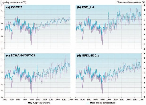
Very few of the examined model outputs showed cooling or no change. The exception in the analysis is Reykjavik, Iceland. The CGCM2 and GFDL-R30_C scenarios for the grid cell that contains Reykjavik project mean annual and summer (May–August) [[temperature]s] that generally are not warmer than 20^th-century observations, and temperatures at the end of the 21^st century that are near the long-term means of the recorded data (Fig. 14.6a,d). Other model scenarios for the Reykjavik grid cell generally show a warming trend (Figs. 14.6b,c), but the magnitude is notably less than most of the other grid cells and stations examined. The four scenarios shown in Fig. 14.6 produce higher values of both summer and mean annual temperature than were recorded during the mid-20^th century temperature peak, but in this highly maritime area none of the scenarios greatly exceed the mid-20^th century temperatures. Note the variability in the degree to which the different scenarios reproduce the historical relationship between the two variables depicted.

Variability and seasonality (14.4.4)

In addition to long-term trends and magnitudes of temperature increase, the models produce different features of shorter-term climate variability. Often these short-term climate events or minor trends can be decisive ecological influences. For example, even one or two years of high temperatures can be enough to produce extreme risk of forest fire^[6] or optimal conditions for major outbreaks of insects that kill trees or reduce their growth (Section 14.8 (Use and evaluation of the ACIA forest and agriculture scenarios)). Conversely, cold spells during the growth season may harm or kill the trees. A short-term period of favorable weather may trigger production of especially large tree seed crops, with long-lasting ecological consequences^[7]. The stations used for scenario analysis exhibit the opposite temperature relationships mentioned in Section 14.2.4 (Use and evaluation of the ACIA forest and agriculture scenarios) (Fig. 14.7). When summer (June–August) temperatures are high at Fairbanks, Alaska (western interior of North America) they tend to be low at Yakutsk, Russia (eastern interior of Eurasia) (Fig. 14.7a). When mean annual temperatures at Goose Bay, Labrador, Canada (eastern edge of North America) are high, they tend to be low at Haparanda, Sweden (western edge of Eurasia) (Fig. 14.7b).

Because these features of climate variability are so important in producing ecological effects, it is important to understand the behavior of the models with respect to key features of short- and medium-term variability and seasonality.

Most of the ACIA-designated model outputs for the grid cells examined reproduce something close to the historical record of the difference between summer and mean annual temperature (Figs. 14.6 and 14.8a,c,d,e). However, sometimes scenario outputs show a different relationship between summer (May–August) and mean annual temperature than do the recorded data (Fig. 14.8b). All the model scenarios shown in Fig. 14.8 project temperature increases that are likely to substantially alter the moderately temperature-limited forest climate typical of the 20^th century. The models project temperature ranges that would surpass thresholds for key factors such as outbreaks of insects that attack trees, new species, and altered ecosystem functions such as growth, fire (Climate change and fire in the Arctic), and decomposition.

The CGCM2 projections for the grid cell containing Fairbanks, Alaska, do not reproduce the same relationship between temperature trends in the coldest winter months and mean annual temperature as the recorded data (Fig. 14.9), and this disparity widens with time. It is possible that climate change would actually produce such an effect, but not all the scenarios agree on such features and realistic projections of effects on forests and agriculture require the resolution of such discrepancies. Different models have different strengths and weaknesses and all should be applied with an awareness of their limitations, circumstances in which they perform well, and novelties that could affect assessments of key climate-dependent processes. Differences in the relationship between seasonal and annual climate variables can have particular ecological importance. For example, a higher growing-season temperature may increase the growth of trees, leading to one set of effects, but an increasing mean annual temperature may promote thawing of permafrost (Permafrost in the Arctic), which could undermine or destroy the soil rooting zone for trees growing on such sites. Thus, different rates of temperature increase (annual versus seasonal) may produce quite different ecological effects.

"Surprises" in climate change effects (14.4.5)

As with any use of models to project the future, a note of caution must be introduced. The projections of climate change and impacts on forests, land management, and agriculture are only as good as the climate models upon which they are based. It is also important to understand that the consequences of change introduced into [[ecosystem]s] often include elements of chance and contingency that have very real and long-lasting consequences. Even though ecological events could unfold in a variety of ways under a given climate scenario, when events do take a certain pathway of cause and effect, this closes off another set of outcomes from that point onward. These elements of chance and contingency make it difficult to project ecosystem responses. However, other elements can assist in the projection of ecosystem responses. Including large areas in the analysis allows processes that have a variety of potential outcomes (e.g., the number of trees of a certain species reproducing successfully after a fire (Climate change and fire in the Arctic)) to occur repeatedly. Any process that expands the pool of possible outcomes (either simulated outcomes or those that can be measured in ecosystems) of the climate change "experiment" will then cause the results or outcomes to begin to approach some distribution that may be described. Repeated outcomes can be produced not only as the result of multiple examples across space, but as the result of multiple outcomes across time in the same place. As a result, when larger areas and longer periods of analysis are involved, the outcomes in ecosystems can be better described.

The climate changes that are the most difficult to project are low-probability, high-impact events. By definition, there are few examples of such events to learn from; in fact, analogous events may not have occurred during the period of the observational record. An example in forest ecosystems is the introduction and spread of tree pathogens such as insects or fungi. Newly introduced pathogens are capable of radically reducing the abundance of susceptible trees, with long-lasting consequences, yet there is no direct human experience of such events and no evidence of the influence of such outbreaks in the past. Temperatures maintain the current distribution limits of many of these insect and disease pathogens, so if temperatures increase, then movement of new pathogens into the northern boreal forest (Arctic boreal forest environments) is highly likely. Temperature increases in the boreal region can also increase the risk of freezing damage. Boreal forest vegetation is generally well adapted to survive or recover from brief periods of below-freezing temperatures after the initiation of growth in the spring. However, some of these freeze-protection mechanisms provide protection from temperatures only slightly below freezing or are not fully effective at the earliest stage of growth. Earlier initiation of growth in the spring or even in the late winter in the boreal forest as the result of increasing temperatures is very likely to be followed by a return to seasonal cold temperatures well below freezing, resulting in damage that would not occur with later emergence from winter dormancy^[8]. The upper levels of temperature increases projected by the five ACIA-designated models are within the range of climate change that is likely to include "ecosystem surprises" for which no historic analogue exists and which ecological modeling is not likely to project.

However, humans are not passive spectators of change in forest [[ecosystem]s] or forest resources that are important to them. Humans actively intervene, plan, and manage forest resources and agents of change in forests through their influence on factors such as fire that affect forests and forest values. Humans completely plan and create agricultural crops, livestock herds, and marketing systems. Therefore, it is possible for climate change to initially create effects that humans can respond to in a way that makes humans the most important agent of change. In some ways, these management responses are part of the standard set of land and resource management treatments that forestry and agriculture have developed over time. Reforestation, new species plantations, salvage of dead trees, sanitation treatments of a stand to reduce its vulnerability to pathogens, planting new crops, and altering soil or site conditions have a long history. Crops can be moved to suitable temperature zones, fields irrigated, and tillage systems adjusted to manipulate soil temperature within certain limits. What is new, and only now being developed, is the application of these techniques and the development of additional techniques to achieve specific goals associated with climate change in the far north, including both adaptation and mitigation approaches, and some appreciation of the associated costs.

Differences between the B2 and A2 emissions scenarios (14.4.6)

For all of the model analysis presented in this chapter, projections based on the B2 emissions scenario (Section 4.4.1 (Use and evaluation of the ACIA forest and agriculture scenarios)) were used. This section evaluates the possible differences between model projections based on the A2 emissions scenario and those based on the B2 emissions scenario.

Broadly speaking, all the ACIA-designated models forced with either emissions scenario project that [[temperature]s] within the boreal region will reach levels higher than shown by reconstructions of climate for nearly the last 1,000 years or essentially since the Medieval Warm Period. In every case, the models forced with the A2 emissions scenario project higher temperatures at the end of the 21^st century than they project when forced with the B2 emissions scenario (Section 4.4.2 (Use and evaluation of the ACIA forest and agriculture scenarios)). The temperature increase over the 21^st century projected by the model with the least warming when forced with the B2 emissions scenario (CSM_1.4) is about 3.5°C, but the same model when forced with the A2 emissions scenario projects a temperature increase of about 4.5°C over the same period. The greatest temperature increase over the 21^st century – slightly more than 7°C – is projected by the ECHAM4/OPYC3 model forced with the A2 emissions scenario.

Considered from the broadest perspective, the difference between projections based on the A2 emissions scenario versus those based on the B2 emissions scenario is largely a matter of timing of effects on forests (Climate change and forest distribution in the Arctic) rather than different kinds of effects. In practical terms, this means that the thresholds described in this chapter would be reached sooner under climate conditions projected using the A2 emissions scenario compared to conditions projected using the B2 emissions scenario. The difference in timing of these effects is projected to be as much as 40 years earlier in the case of the projections based on the A2 emissions scenario. The temperature projections of each model when forced with the A2 emissions scenario begin to diverge from projections using the B2 emissions scenario in amounts significant for forest processes after about 2040.

In general, the projections of the ECHAM4/OPYC3 model forced with the B2 emissions scenario best matched the features of annual temperature variability in the recorded data for the stations examined in this chapter; most of the other four scenarios produced less annual variability. The ECHAM4/OPYC3 model forced with the A2 scenario projects a pattern of steep temperature rise early in the 21^st century, then a period of little change, and finally a steep rise again in the last decades of the century. This suggests that the effects of climate change under this scenario, with large variability possible from year to year, could be especially sudden. Under such a scenario the risk of extreme events, such as widespread forest fires and insect outbreaks, would probably be greatest.

Chapter 14: Forests, Land Management, and Agriculture (Use and evaluation of the ACIA forest and agriculture scenarios)
14.1. Introduction (Use and evaluation of the ACIA forest and agriculture scenarios)
14.2. The boreal forest: importance and relationship to climate
14.3. Land tenure and management in the boreal region
14.4. Use and evaluation of the ACIA scenarios
14.5. Agriculture (Agriculture in the Arctic)
14.6. Tree rings and past climate
14.7. Direct climate effects on tree growth
14.8. Climate change and insects as a forest disturbance
14.9. Climate change and fire
14.10. Climate change in relation to carbon uptake and carbon storage
14.11. Climate change and forest distribution
14.12. Effects of ultraviolet-B on forest vegetation
14.13. Critical research needs

References

Citation

Committee, I. (2012). Use and evaluation of the ACIA forest and agriculture scenarios. Retrieved from http://editors.eol.org/eoearth/wiki/Use_and_evaluation_of_the_ACIA_forest_and_agriculture_scenarios