Regional climate change assessment
| Topics: |
Our climate varies regionally, and the temperature and precipitation tend to be influenced by local geographical characters such as latitude, altitude, distance from the coast, nearby ocean currents, prevailing winds, mountain ranges and vegetation. Different local and regional climate characteristics were classified by Köppen in the early 20th Century. The regional climate has a key role in determining soil type, ecosystem type distibution, hydology, erosion processes etc. Changes in regionalclimate alter the fabric of our physical environment.
A global climate change will have various implications for the local weather statistics (local climate characteristics), but the local climate response will differ from place to place. The local information is important when one wants to study the impacts of a climate change or implement an adaption strategy. How will the rainfall statistics be affected where I live? Is the drainage system adequate? Do the reservoir dams have sufficiently large capacity to buffer droughts? Will the drainage system be able to cope with future rainfall extremes? How much will the local temperature rise? Will high winter temperatures have any implications for the snow conditions? Is the storm (Tropical weather and hurricanes) statistics going to change along the coast? These are but some questions that only can be answered with detailed local climate information.

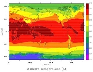
Global Climate models (GCMs) can be used to make projections for large-scale aspects of the climate, but they alone are not yet able to provide accurate and detailed description of the local characters. The reason why the GCMs are not able to provide an accurate description of the local climate is that the planet is represented by a coarse mesh of grid-point values with ~100-300 kilometers (km) between each point (varies with the latitude). The computer resources (memory and speed) are still not sufficient for using global coupled climate models with high spatial resolution to capture a high degree of spatial details. Thus the spatial resolution is about ~100-300 km. In addition, the models represent small-scale phenomena by simpler statistical models and solve the dynamics equations discretely though various numerical methods, both which may lead to biases on the smallest grid-box scales.
Despite the GCMs' inability to give a detailed picture when it comes to local scales, it is possible to infer likely local response to a change on larger scales over the same area. It is well known that the local climate is influenced by the nearby geography ('physiography') and the large-scale climatic conditions in which it is embedded (spatial scales of ~1,000 km).
The procedure of estimating the response at local scales from larger scales is known as 'downscaling'

There are two main methods for deriving information about the local climate: (i) dynamical downscaling (also referred to as 'nested modeling' using 'regional climate models' or 'limited area models') and (ii) statistical downscaling (also referred to as 'empirical' or 'statistical-empirical' downscaling).
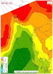
Dynamical downscaling involves a regional atmospheric model in a similar fashion to ordinary day-to-day numerical weather forecasting. These models are built on laws of physics (Navier-Stokes equations, thermodynamics (Laws of thermodynamics), ideal gas law, etc). The main difference is that a regional climate model (RCM) is more concerned about slow changes in the boundary conditions (changes in the atmospheric composition, e.g. CO2) than the exact description of the initial conditions used for the simulations.
Dynamical downscaling can in principle yield a wide range of climate elements over a large region, but these data are merely the product of a model and are not perfect. It is therefore important to validate the model against real observations.
Caveats associated with RCMs include inconsistency between the driving GCM and RCM in terms of describing small-scale processes, differences in representing the coupling between the atmosphere and ocean/land surface, spurious effects related to lateral boundaries (numerical waves or ill-conditioned solutions to the mathematical equations), or inconsistencies in how improved representation of small scale phenomena affect the ambient climate (e.g. cyclones play a role in heat transport, both vertically and laterally, and improved realism may alter the heat transport). Thus, it is important to compare results from RCMs with independent methods whenever possible (e.g. statistical downscaling).
Statistical downscaling involve statistical models that have been trained on empirical data. Data representing large-scale atmospheric conditions (predictors) represent one side of the equation and data representing the local parameter (predictand) the other. When these models are developed (or 'trained or 'calibrated'), then a statistical relationship is sought between the predictors and the predictands for the past. These may involve regression, canonical correlation analysis (CCA), analogs, neural nets, and may involve everything from simple indices to advanced multivariate methods (linear algebra).

It is important that the predictors can be reproduced skilfully by the GCMs, so that the statistical models can be 'ported' to climate model results. It is also important that the a climate change can be seen in the predictor (i.e. the predictor captures the climate signal), and that the relationship between the predictor and predictand is constant for the future. These assumptions are not guaranteed. Furthermore, the statistical models do not provide a perfect reproduction of the local element. Thus, it is important to compare these results with other independent downscaled results whenever possible (e.g. dynamical downscaling or other types of statistical downscaling).
Empirical data are important both for calibrating the models and for validating them. The validation of the models involves comparing the model output to independent data not used for the model construction. Note, there are many ways to apply statistical models to data, but many may be inappropriate for the case in question. Therefore, it is important to have a thorough understanding of the problem and the models (their limitations) when using these to study local climate changes.
Often RCMs do not provide data that are close to the observed values. The RCMs provide a mean value for a box (e.g. 25 km by 25 km by 10 meters) whereas the observations are point measurements. Furthermore, the climatic elements may vary strongly over short distances in regions with complex terrain. Thus, it is common to apply a statistical correction to RCM data before using these for impact studies. Sometimes, the correction may resemble simple statistical downscaling in the sense that both involve a statistical model with a set of limitations.
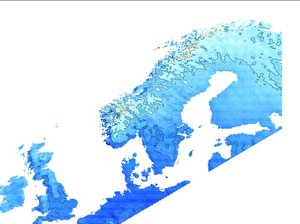
Statistical downscaling typically yields results for a single site, but it is possible to assemble the information from several sites in order to make maps (e.g. using so-called Geographical Information Systems, or GIS).
Further Reading
- IPCC 2007, Chapter 11.
- IPCC 2001, Chapter 10.
- Why global climate models do not give a realistic description of the local climate.
- Regional Climate Projections RealClimate.org.
- Compendium on Empirical-Statistical Downscaling used at the STATME summerschool in Lodz, Poland, June 2007.
