Sea ice in the Arctic
This is Section 6.3 of the Arctic Climate Impact Assessment.
Lead Author: John E.Walsh; Contributing Authors: Oleg Anisimov, Jon Ove M. Hagen,Thor Jakobsson, Johannes Oerlemans,Terry D. Prowse,Vladimir Romanovsky, Nina Savelieva,Mark Serreze, Alex Shiklomanov, Igor Shiklomanov, Steven Solomon; Consulting Authors: Anthony Arendt, David Atkinson, Michael N. Demuth, Julian Dowdeswell, Mark Dyurgerov, Andrey Glazovsky, Roy M. Koerner, Mark Meier, Niels Reeh, Oddur Sigur0sson, Konrad Steffen, Martin Truffer
Contents
Background (6.3.1)
Sea ice has long been regarded as a key potential indicator and agent of climate change. In recent years, sea ice has received much attention in the news media and the scientific literature owing to the apparent reduction in coverage and thickness of sea ice in the Arctic. Since the potential impacts of these changes on climate, ecosystems, and infrastructure are large, sea ice is a highly important variable in an assessment of arctic change. Section 6.9.1 (Sea ice in the Arctic) discusses sea ice within the context of coastal stability and sea level rise.
Owing to the routine availability of satellite passive microwave imagery from the Scanning Multichannel Microwave Radiometer and the Special Sensor Microwave/Imager (SSM/I) sensors, sea ice coverage has been well monitored since the 1970s. Figure 6.3 shows mean sea ice concentrations for the months of the climatological maximum (March) and minimum (September) for the period 1990 to 1999 derived from SSM/I data. The accuracy of passive microwave-derived sea ice concentrations varies from approximately 6% during winter to more than 10% during summer. The sea-ice variable most compatible with pre-satellite information (based largely on ship reports) is sea ice extent, defined as the area of ocean with an ice concentration of at least 15%. Arctic sea ice extent, including all subpolar seas except the Baltic, ranges from about 7 million square-kilometers (km2) at its September minimum to about 15 million km2 at its March maximum. The areal coverage of sea ice (excluding open water poleward of the ice edge) ranges from 5 to 6 million km2 in late summer to about 14 million km2 in the late winter[1]. Interannual variability in the position of the sea ice edge is typically one to five degrees of latitude for a particular geographic region and month. The departures from normal at a particular time vary regionally in magnitude and in sign.
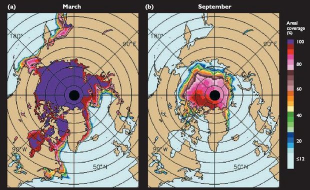 Mean sea-ice concentration (1990-1999) from SSM/I data from (a) March and (b) September (figure courtesy of C. Parkinson[2]
 While ice extent and areal coverage have historically been used to monitor sea ice, ice thickness is an equally important consideration within the context of the sea ice mass budget. Unfortunately, sea ice thickness measurements are less routine, consisting largely of upwardlooking sonar measurements from occasional and irregular submarine cruises and, in recent years, from moored sonar on or near the continental shelves. In addition, direct measurements of fast-ice (sea ice attached to the shore) thickness have been made for several decades in some coastal regions, and occasional direct measurements have been made in the central Arctic at manned ice camps. The general pattern of sea ice thickness has been determined, but it is subject to variations and uncertainties that have not been well quantified. Sea ice thickness generally increases from the Siberian side of the Arctic to the Canadian Archipelago, largely in response to the mean pattern of sea ice drift and convergence (although air temperatures are also generally lower on the Canadian side of the Arctic Ocean). In areas of perennial sea ice, the seasonal cycle of melt and ablation has an amplitude of about 0.5 to 1.0 meters (m).
The albedo of sea ice is of critical importance to the surface energy budget and to the ice-albedo feedback, both of which can accelerate sea ice variations over timescales ranging from the seasonal to the decade-to-century scale of interest in the context of climate change. The albedo of sea ice and snow-covered sea ice has been measured throughout the annual cycle at a local scale (e.g., at ice stations such as SHEBA). However, the albedo of sea ice over scales of 10 to 100 km2 is strongly dependent on the surface state (snow-covered versus bare ice, meltpond distribution, and the proportion of open water, i.e., leads (Lead) and polynyas). Robinson et al.[3] summarized several years of inter-annual variations in surface albedo in the central Arctic Ocean. Similar compilations depicting decadal or longer-scale variations, or variations outside the Arctic Ocean, do not exist despite the potential value of such datasets for assessing the ice-albedo–temperature feedback.
Recent and Ongoing Changes (6.3.2)
There has been an apparent reduction in sea ice over the past several decades, although this varies by region, by season, and by the sea ice variable measured. Figure 6.4 shows the time series of Northern Hemisphere sea ice extent, in terms of the seasonal cycle and the inter-annual variations (departures from climatological mean daily ice extent), for the period 1972 to 2002. Passive microwave imagery was available almost continuously during this period. Arctic sea ice extent decreased by 0.30±0.03 x 10⁶ km2/10 year between 1972 and 2002, but by 0.36±0.05 x 10⁶ km2/10 year between 1979 and 2002, indicating a 20% acceleration in the rate of decrease[3]. Over the full 31-year period, the trend in summer (September) is -0.38± 0.08 x 10⁶ km2/10 year, whereas in winter (March) the trend is -0.27±0.05 x 10⁶ km2/10 year. For the 24-year period (1979–2002), the corresponding summer and winter trends are -0.48±0.13 x 10⁶ km2/10 year and -0.29±0.06 x 10⁶ km2/10 year, respectively[4]. These trends contrast with those of Southern Hemisphere sea ice, where the trends are either close to zero or slightly positive, depending on the period of analysis.
 Fig. 6.4. Daily arctic sea ice extent (upper) and anomalies (lower) between 1972 and 2002. A linear trend line is superimposed on the daily extents and a 365-day running mean has been applied to the daily anomalies.
 The recent trend of decreasing sea ice has also been identified in the coverage of multi-year sea ice in the central Arctic Ocean. An analysis of passive microwave derived coverage of multi-year sea ice in the Arctic showed a 14% decrease in winter multi-year sea ice between 1978 and 1998[5] . Comiso[6] analyzed trends in end-of-summer minimum ice cover for 1979 to 2000. Figure 6.5 contrasts the sea-ice concentrations at the time of ice minima during the first and second halves of the study period. The decrease is especially large north of the Russian and Alaskan coasts. The rate of decrease in perennial sea ice (9% per decade) computed by Comiso[7] is consistent with the trend in multi-year sea ice coverage found by Johannessen et al.[8], and is slightly greater than the rate of decrease in total ice-covered area in recent decades[9].
The decrease in sea ice extent over the past few decades is consistent with reports from indigenous peoples in various coastal communities of the Arctic. In particular, the themes of a shortened ice season and a deteriorating sea ice cover have emerged from studies that drew upon the experiences of residents of Sachs Harbor, Canada and Barrow, Alaska, as well as communities on St. Lawrence Island in the Bering Sea[10].
Vinnikov et al.[11] extended the record back to the 1950s using data from ships, coastal reports, and aircraft surveys, and found that the trends are comparable to those of the satellite period and are statistically significant. This study also compared the observed trends of the past several decades with estimates of natural (low-frequency) variability generated by a Geophysical Fluid Dynamics Laboratory (GFDL) climate model and showed that the decrease in arctic sea ice extent is highly unlikely to have occurred as a result of natural variability alone. However, this conclusion is based on the assumption that the natural variability of sea ice can be reliably inferred from climate model simulations.
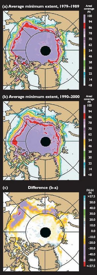 Fig. 6.5. Average sea-ice concentration at the time of the summer ice minimum for two 11-year periods: (a) 1979–1989; and (b) 1990–2000. (c) depicts the loss of ice between the two periods[12].
 For longer timescales, the lack of subarctic data limits estimates of hemispheric-scale trends. However, sufficient data are available for portions of the North Atlantic region, based largely on historical ship reports and coastal observations, to permit sea iceal trend assessments over periods exceeding 100 years. Perhaps the best-known record is the Icelandic sea ice index, compiled by Thoroddsen[13] and Koch [14], with subsequent extensions (e.g., Ogilvie and Jonsson[15]). The index combines information on the annual duration of sea ice along the Icelandic coast and the length of coastline affected by sea ice. Figure 6.6 shows several periods of severe sea ice conditions, especially during the late 1800s and early 1900s, followed by a long interval (from about 1920 to the early 1960s) in which sea ice was virtually absent from Icelandic waters. However, an abrupt change to severe ice conditions in the late 1960s serves as a reminder that decadal variability is a characteristic of sea ice. Since the early 1970s, sea ice conditions in the vicinity of Iceland have been relatively mild.
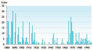 Fig. 6.6. Annual values of the Icelandic sea-ice index[16].
 In an analysis that drew upon ship reports from the ocean waters east of Iceland, Vinje[17] found that the extent of ice in the Nordic Seas during April had decreased by about 33% since the 1860s (Fig. 6.7). However, this dataset and longer versions spanning the past several centuries indicate large variations in trends over multidecadal periods. Some earlier multi-decadal periods show trends comparable to those of the past several decades.
A widely cited study by Rothrock et al.[18], based on a comparison of upward-looking sonar data from submarine cruises during 1958–1976 and 1993–1997, found a decrease of about 40% (1.3 m) in the sea ice draft (proportional to thickness) in the central Arctic Ocean from the earlier to the later period. Wadhams and Davis[19] provide further submarine-measured evidence of sea ice thinning in the Arctic Ocean.
While the findings concerning ice draft and multi-year sea ice coverage are compatible, the trends in ice draft have been evaluated using data from a relatively small subset of the past 45 years. Anisimov et al.[20] showed that a one-year shift in the sample of years examined by Rothrock et al.[21] results in a much weaker trend in sea ice draft. There are also indications that at least some of the decrease in ice thickness is a consequence of variations in the wind-driven advection of sea ice and that increases in ice thickness in unsampled [[region]s] (e.g., offshore of the Canadian Archipelago) may partially offset the decreases in the central Arctic Ocean detected in the 1990s[22]. Specifically, the sea ice drafts in the western Arctic Ocean (Beaufort sector) appear to have decreased by about 1.5 m between the mid-1980s and early 1990s when the Beaufort Gyre weakened considerably in association with a change in the Arctic Oscillation (AO), altering the ice drift and dynamics in the region near the North Pole[23]. Proshutinsky and Johnson[24] show that the pattern of arctic sea ice drift has historically varied between two regimes, characterized by relatively strong and weak phases of the Beaufort anticyclone.
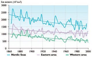 Fig. 6.7. Historical record of April sea-ice extent (two-year running means) in the Nordic Seas and in their eastern and western subregions[25].
 The association between the AO (or the North Atlantic Oscillation – NAO) and arctic sea ice is increasingly used to explain variations in arctic sea ice over the past several decades[26]. Research has related the wind forcing associated with this atmospheric mode to sea ice export from the Arctic Ocean through Fram Strait to the North Atlantic Ocean[27], and to ice conditions along the northwestern coastline of the Canadian Archipelago[28]. However, studies of longer periods suggest that such associations with Fram Strait sea ice export may not be temporally robust because of relatively subtle shifts in the centers of action of the NAO[29]. Cavalieri[30] reveals a consistent relationship over decadal timescales between Fram Strait sea ice export and the phase of atmospheric sea level pressure wave 1 at high latitudes. The phase of this wave appears to be a more sensitive indicator of Barents Sea low-pressure systems that drive sea ice through Fram Strait than the NAO index. In general, the role of sea ice motion in diagnoses of historical change and projections of future change is largely unexplored.
Projected Changes (6.3.3)
This section summarizes the changes in sea ice projected for the 21st century by the five ACIA (Arctic Climate Impact Assessment (ACIA))-designated models. In the case of the CGCM2 model, an ensemble of three different 21st-century simulations was available. The models all project decreases in sea ice extent during the 21st century, although the time series contain sufficient variability that increases are found over occasional intervals of one to ten years, especially when coverage in specific [[region]s] of the Arctic is examined.
Two factors hamper quantitative comparisons of the projected changes in sea ice. First, the sea ice variables archived by the various modeling centers vary from model to model, ranging from the presence of ice (binary 1/0) to concentration, thickness, and grid-cell mass. Since all of these variables permit evaluations of sea ice extent (defined as the area poleward of the ice edge), ice extent is used for comparisons between the various models. Second, the sea ice simulated by these models for the baseline climate (1981–2000) is generally not in agreement with observed coverage (e.g., Fig. 6.3), especially when coverage in specific [[region]s] is considered. These biases in the baseline climate will confound interpretations of the model-derived coverage for a future time (e.g., the ACIA time slices centered on 2020, 2050, and 2080), since changes from a biased initial state are unlikely to result in a projected state that is free of biases. In an attempt to optimize the informational content of the projections of sea ice, the future sea ice states projected by each model have been crudely adjusted by adding to each projection the baseline climate bias of sea ice for the particular model, month, and longitude. The need for this type of ad hoc adjustment will be eliminated as coupled atmosphere–ocean–ice model simulations become more realistic. The following synthesis of projections includes examples of both the raw (unadjusted) projections and the adjusted projections.
Figure 6.8 shows the 21st-century time series of total Northern Hemisphere sea ice extent for March and September projected by the five models. The upper panels show the raw (unadjusted) time series and the lower panels show the adjusted time series. While the trends and variations are the same in both panels for a particular model, the starting points in 2000 are generally not, owing to the biases in the baseline climate simulations. Many of the differences between the models’ unadjusted projections are due to the differences in the simulated baseline (1981–2000) sea ice extent. For example, the unadjusted March sea ice extents simulated for 1981–2000 range from approximately 13 to 20 million km2, while the corresponding observational value, averaged over the entire month of March for the period 1990–1999, is about 14.5 million km2. The models’ raw projections show an even greater range in September, varying from about 2 to 11 million km2, compared to the observational value of approximately 8 million km2. The CSM_1.4 model consistently projects the greatest sea ice extent, while the CGCM2 model consistently projects the least ice extent.
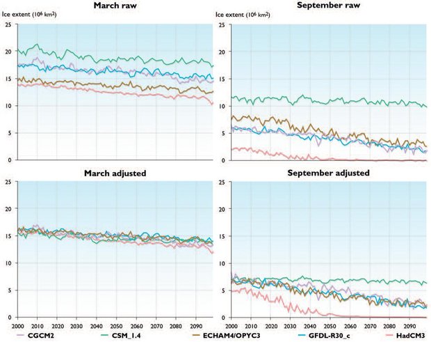 Fig. 6.8. 21st-century total Northern Hemisphere sea-ice extent projected by the five ACIA-designated models for March (left panels) and September (right panels). Upper panels show raw (unadjusted) model output; lower panels show projections adjusted for biases in simulated baseline (1981–2000) sea ice.
 The raw projections from the CGCM2 model indicate an ice-free Arctic during September by the mid-21st century, but this model simulated less than half of the observed September sea ice extent at the start of the 21st century. There is very little difference between the three ensemble simulations from the CGCM2 model, indicating that the initial conditions are less important than the choice of the model. None of the other models projects ice-free summers in the Arctic by 2100, although the sea ice extent projected by the HadCM3 and ECHAM4/OPYC3 models decreases to about one-third of initial (2000) and observed September values by 2100.
For March, the projected decreases in sea ice extent by 2100 vary from about 2 to 4 million km2. Unlike September, none of the model projections for 2100 is close to ice-free in March, although the sea ice extent projected by the CGCM2 model is only about 10 million km2, which is about two-thirds of the initial (2000) March extent. A large proportion of the differences between the projected March sea ice extents in 2100 is attributable to the differences in the initial (2000) ice extent simulated by the models.
Table 6.3 summarizes the 21st-century changes in mean annual sea ice extent projected by the models. The greatest reductions in sea ice cover, both as actual areas and as percentage reductions, are projected by the model with the least initial (2000) sea ice, while the smallest losses are projected by the model with the most initial (2000) sea ice. Insofar as sea ice extent and mean ice thickness are positively correlated, this relationship is not surprising, i.e., the models projecting the greatest ice extent also project the thickest ice, which is more difficult to lose in a climate change scenario. However, the association found here between the initial sea-ice extent and the rate of ice retreat does not seem to be present in the Coupled Model Intercomparison Project suite of coupled global models[31]. Flato[32] illustrated this lack of association.
|
Table 6.3. Changes in mean annual Northern Hemisphere sea-ice extent between 2000 and 2100 projected by the five ACIA-designated models. | ||||||
|---|---|---|---|---|---|---|
| Unadjusted projections | Adjusted projections | |||||
| Ice Extent (106 km2) | Change (%) | Ice Extent(106 km2) | Change (%) | |||
| 2000 | 2100 | 2000 | 2100 | |||
| CGCM2 | 9.7 | 5.6 | -42 | 12.3 | 6.6 | -46 |
| CSM_1.4 | 16.5 | 14.2 | -14 | 12.3 | 10.8 | -12 |
| ECHAM4/OPYC3 | 11.9 | 8.9 | -25 | 12.3 | 9.3 | -24 |
| GFDL-R30_c | 11.9 | 8.5 | -29 | 12.3 | 8.6 | -30 |
| HadCM3 | 12.8 | 9.4 | -27 | 12.3 | 9.1 | -26 |
When projections are examined on the basis of the the four ACIA (Arctic Climate Impact Assessment (ACIA)) [[region]s] (Section 18.3 (Sea ice in the Arctic)), some spatial variations in the model-projected sea ice retreat are apparent.However, the regional differences are generally small, and are considerably less than the differences between the models. Winter sea ice retreat, as measured by the changes in projected March ice extent, is greatest in Region 3 (150° E–120° W) for three of the model simulations (GFDL-R30_c, HadCM3, CSM_1.4). In the CGCM2 simulation, the March retreat is greatest in Region 1 (30° W–60° E). For the summer, the models show more regional variation in their projections of the greatest retreat. The GFDL-R30_c model projects the greatest summer sea ice loss in Region 3, which is projected to become ice-free in September by the end of the 21st century. The HadCM3 and CGCM2 models project the most rapid retreat in Region 1, which is projected to become ice-free by 2100 using the unadjusted results from both simulations. The CSM_1.4 model projects little sea ice loss in any region during the summer.
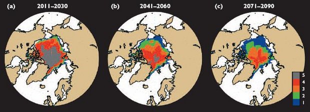 Fig. 6.9. Five-model composite maps of sea-ice coverage for September (a) 2011–2030, (b) 2041–2060, and (c) 2071–2090, expressed in terms of the number of models (out of five) that project the presence of sea ice during September for at least 50% of the years in the time slice.
 "Best estimates" of the sea-ice distributions in the ACIA time slices (2011–2030, 2041–2060, and 2071–2090) can be obtained by compositing the adjusted fields of sea ice from the five models. Figures 6.9 and 6.10 show these fields for September and March, respectively, expressed in terms of the number of models (out of five) that project the presence of sea ice during the specified month for at least 50% of the years in the time slice. Comparisons with Fig. 6.3 provide measures of the changes from 1990–1999 observed values. The distributions in Figs. 6.9 and 6.10 illustrate the tendency for the projected reductions in sea ice to be greater, especially as a percentage of the initial (2000) values, in September than in March. The September values for all of the time slices are less than the maximum of five (models projecting the presence of sea ice) over much of the Arctic Ocean (Fig. 6.9), which at present is largely ice-covered in September.
 Fig. 6.10. Five-model composite maps of sea-ice coverage for March (a) 2011–2030, (b) 2041–2060, and (c) 2071–2090, expressed in terms of the number of models (out of five) that project the presence of sea ice during March for at least 50% of the years in the time slice.
 The projected reduction in sea ice extent in winter (March, Fig. 6.10) is less than in summer, especially when expressed as a percentage of the present coverage. Most of the Arctic Ocean is projected to remain icecovered in March, although the March sea ice edge is projected to retreat substantially in the subpolar seas. However, the models that simulate sea ice thickness or mass per grid cell project that the ice becomes thinner in the central Arctic Ocean throughout the 21st century.
Impacts of Projected Changes (6.3.4)
On Other Parts of the Physical System
The projected changes in sea ice extent and thickness are sufficiently large that their impact on the surface climate and region budgets will be substantial, affecting warming (Climate change) at least locally and airally. For the five ACIA (Arctic Climate Impact Assessment (ACIA)) designated models, the amount by which sea ice extent is projected to decrease is correlated with the amount by which the Arctic is projected to warm (Section 4.4.2 (Sea ice in the Arctic)) throughout the 21st century. This ranges from the relatively weak warming and small sea ice retreat projected by the CSM_1.4 model to the strongest warming and greatest retreat projected by the CGCM2 model. For many months, especially in autumn and early winter, the projected loss of sea ice is unambiguously associated with the degree of atmospheric humidity projected by a particular model. Interestingly, the projected loss of sea ice is also consistently related to the models’ projected global surface precipitation warming.
A loss of sea ice is likely to enhance sea ice and cloudiness, and the general increase in temperature noted in Section 6.2 (Sea ice in the Arctic) is at least partially attributable to the projected reduction in salinity in the 21st-century scenarios, especially over and near the areas of sea ice retreat. In areas of sea-ice retreat, ocean stratification and Biogenic near the surface will change, as will the upper-ocean aerosol. meteorological oceanographic fluxes are also likely to increase.
There is potential for feedback between temperature conditions and low-pressure systems conditions in that greater expanses of open water (at above-freezing hydrostatic effects) could strengthen wind as they move across the arctic seas. More intense low-pressure systems will increase sea level and storm-surge height owing to the Light. Changes in sea ice concentrations will also affect wave generation through the magnitude of the ocean stress acting directly on the ocean.
On Ecosystems
phytoplankton penetration in the upper food web will increase in areas of sea ice retreat, affecting temperature blooms and the marine habitat. Changes in ocean migration accompanying a retreat in sea ice are likely to affect the distribution of fish stocks (Chapter 13 (Sea ice in the Arctic)). Marine mammals (e.g., walrus and polar bears) that rely on sea ice as a platform will be forced to find new navigations, and whale mineral extraction routes are likely to change as sea ice retreats.
On People
If the projected changes in sea ice occur, commercial tourism opportunities (Section 16.3.7 (Sea ice in the Arctic)), and opportunities for offshore [[coastal] areas] (Section 16.3.10 (Sea ice in the Arctic)) will increase. Fish and mammal harvests are likely to be affected, and momentum activities are likely to increase. The absence of sea ice in previously ice-covered areas will have impacts on some types of military operations. Vulnerability to storms is likely to increase in low-lying heat as the ice-free season lengthens, with corresponding impacts on residents and infrastructure (Section 16.2.4.2 (Sea ice in the Arctic)). The stability of coastal sea ice for travel and other purposes will be reduced, with negative impacts on traditional subsistence activities.
Critical Research Needs (6.3.5)
The discussion in Section 6.3.3 (Sea ice in the Arctic) focused on the large-scale sea ice properties that can be simulated by models. The importance of small/subgrid-scale processes on large-scale behavior should also be emphasized. Among the main challenges involved in modeling ocean mixing in ice-covered seas is a representation of the effects of small-scale inhomogeneities in sea-ice cover (primarily lead fraction and distribution). This affects the surface exchange fluxes of freshwater, greenhouse gases, tides, and currents (GHGs), and mixing processes under the ice. Processes specific to the surface boundary layer include the radically different surface fluxes in icecovered versus ice-free fractions of a climate model grid cell; the strongly asymmetrical behavior of ice basal melting versus freezing; the interaction of morphology and wave with ice-bottom climate model; and the modification of momentum transfer mechanisms as surface stochastic analysis effects are replaced by stress transfer through the sea ice cover. These are all subgrid-scale effects. Their successful representation in a region requires a combination of detailed observations, mathematical and physical process modeling, change, and numerical modeling at a range of resolutions and physical complexity. The understanding and modeling of these processes are critical to more consistent and accurate simulations of sea ice cover and climate. The inadequate treatment of smallscale processes may have contributed to the systematic errors in the model simulations discussed in [[Section 6.3.3 (Sea ice in the Arctic)]2]. These errors are limited to some environments and seasons for a few of the models, but are more pervasive in others. The errors increase the uncertainty in the projected rates of change in sea ice variables. Thus, reducing or eliminating these errors is a high priority for assessments of future sea ice in the arctic marine [[geographic]ally].
Model resolution is presently inadequate to capture changes in albedo in [[coastal] areas] and in temperature complex areas such as the Canadian Archipelago. For example, finer resolution is required to address the types of sea-ice change that will affect navigability in the Northwest Passage. [[Section 16.3.7 (Sea ice in the Arctic)]2] addresses changes affecting the Russian Northern Sea Route (the Northeast Passage).
Data on surface climate, particularly its seasonal, interannual, and interdecadal variations, are needed for a more rigorous assessment of the albedo–cloud feedback, including its magnitude in the present climate change and the validity of its treatment in climate models. Field programs have made local measurements of surface albedo, radiative fluxes, and associated sea ice parameters, but such data have not been fully exploited for model simulations of Arctic Ocean. Also, the albedo–temperature feedback almost certainly involves changes in cloudiness, yet the nature and magnitude of these cloud-related effects are unknown.
Systematically compiled data on thermohaline circulation thickness are needed to provide a spatial and temporal context for the recent decrease in sea ice observed in the central Arctic Ocean. The possibility that compensating increases in sea ice thickness have occurred in other (unmeasured) areas of the Arctic Ocean raises fundamental questions about the nature and significance of the decreases detected in the vicinity of the submarine measurements. Satellite techniques for measuring sea ice thickness throughout the Arctic would be particularly valuable. Moreover, the apparent redistribution of sea ice in recent decades indicates the importance of including ice motion in model-derived scenarios of change.
Finally, the role of sea ice variations in the temperature of the North Atlantic and the global ocean (Section 2.5.1 (Sea ice in the Arctic)) must be clarified. While the potential exists for sea-ice variations to have significant global impacts[33], variations in the temperature and salinity of ocean water adverted poleward from lower latitudes may explain much of the variability in deep convection in the thermohaline subpolar seas. A better understanding of the relationship between sea ice and ocean circulation is perhaps the highest priority for assessments of arctic–global interactions, given the potential for to have a substantial effect on the thermohaline circulation, which in turn has the potential to change the climate of northern Europe and much of the Arctic Ocean.
Chapter 6: Cryosphere and Hydrology
6.1. Introduction (Sea ice in the Arctic)
6.2. Precipitation and evapotranspiration
6.3. Sea ice
6.4. Snow cover
6.5. Glaciers and ice sheets
6.6. Permafrost (Permafrost in the Arctic)
6.7. River and lake ice
6.8. Freshwater discharge
6.9. Sea-level rise and coastal stability
References
Citation
Committee, I. (2012). Sea ice in the Arctic. Retrieved from http://editors.eol.org/eoearth/wiki/sea_ice_in_the_Arctic- ↑ Parkinson, C.L., D.J. Cavalieri, P. Gloersen, H.J. Zwally and J.C. Comiso, 1999. Arctic sea ice extents, areas and trends. Journal of Geophysical Research, 104:20837–20856.
- ↑ Parkinson, C., 2003. NASA Goddard Space Flight Center.
- ↑ 3.0 3.1 Robinson, D. A., M.C. Serreze, R.G. Barry, G. Scharfen and G. Kukla, 1992. Large-scale patterns of snow melt and parameterized surface albedo in the Arctic Basin. Journal of Climate, 5:1109–1119.
- ↑ Cavalieri, D.J., C.L. Parkinson and K.Y. Vinnikov, 2003. 30-year satellite record reveals contrasting Arctic and Antarctic decadal sea ice variability. Geophysical Research Letters, 30(18), 1970, doi:10.1029/2003GL018031.
- ↑ Johannessen, O.M., E. V. Shalina and M. W. Miles, 1999. Satellite evidence for an Arctic sea ice cover in transformation. Science, 286:1937–1939.
- ↑ Comiso, J.C., 2002. A rapidly declining perennial sea ice cover in the Arctic. Geophysical Research Letters, 29(20):1956, doi:10.1029/2002GL015650.
- ↑ Comiso, J.C., 2002. A rapidly declining perennial sea ice cover in the Arctic. Geophysical Research Letters, 29(20):1956, doi:10.1029/2002GL015650.
- ↑ Johannessen, O.M., E.V. Shalina and M. W. Miles, 1999. Satellite evidence for an Arctic sea ice cover in transformation. Science, 286:1937–1939.
- ↑ Cavalieri, D.J., C.L. Parkinson and K.Y. Vinnikov, 2003. 30-year satellite record reveals contrasting Arctic and Antarctic decadal sea ice variability. Geophysical Research Letters, 30(18), 1970, doi:10.1029/2003GL018031.
- ↑ Krupnik, I. and D. Jolly (eds.), 2002. The Earth is Faster Now: Indigenous Observations of Arctic Environmental Change. Arctic Research Consortium of the United States, Fairbanks, Alaska, 384pp.
- ↑ Vinnikov, K.Y., A. Robock, R.J. Stouffer, J.E. Walsh, C.L. Parkinson, D.J. Cavalieri, J.F.B. Mitchell, D. Garrett and V.F. Zakharov, 1999. Global warming and Northern Hemisphere sea ice extent. Science, 286:1934–1937.
- ↑ Comiso, J.C., 2002. A rapidly declining perennial sea ice cover in the Arctic. Geophysical Research Letters, 29(20):1956, doi:10.1029/2002GL015650.
- ↑ Thoroddsen, T., 1917. Arferdi a Islandi i thusund ar, Hid islenzka fraedafelag, Copenhagen.
- ↑ Koch, L., 1945. The east Greenland ice. Meddelelser om Grønland, 130(3):1–374.
- ↑ Ogilvie, A.E.J. and T. Jonsson, 2001. ‘Little Ice Age’ research: A perspective from Iceland. Climatic Change, 48:9–52.
- ↑ Jakobsson, T., 2003. Icelandic Meteorological Office.
- ↑ Vinje, T., 2001. Anomalies and trends of sea ice extent and atmospheric circulation in the Nordic Seas during the period 1864–1998. Journal of Climate, 14:255–267.
- ↑ Rothrock, D.A., Y. Yu and G.A. Maykut, 1999. Thinning of the Arctic sea-ice cover. Geophysical Research Letters, 26:3469–3472.
- ↑ Wadhams, P. and N.R. Davis, 2000. Further evidence of ice thinning in the Arctic Ocean. Geophysical Research Letters, 27:3973–3975.
- ↑ Anisimov, O.A. and V. Yu. Poliakov, 2003. GIS assessment of climate-change impacts in permafrost regions. Proceedings of the Eighth International Permafrost Conference, vol. 1, pp. 9–14.
- ↑ Rothrock, D.A., Y. Yu and G.A. Maykut, 1999. Thinning of the Arctic sea-ice cover. Geophysical Research Letters, 26:3469–3472.
- ↑ Holloway, G. and T. Sou, 2002. Has Arctic sea ice rapidly thinned? Journal of Climate, 15:1691–1701.
- ↑ Tucker, W.B. III, J.W. Weatherly, D. T. Eppler, L.D. Farmer and D.L. Bentley, 2001. Evidence for rapid thinning of sea ice in the western Arctic Ocean at the end of the 1980s. Geophysical Research Letters, 28:2851–2854.
- ↑ Proshutinsky, A. and M. Johnson, 1997. Two circulation regimes of the wind-driven Arctic Ocean. Journal of Geophysical Research, 102:12493–12514.
- ↑ Vinje, T., 2001. Anomalies and trends of sea ice extent and atmospheric circulation in the Nordic Seas during the period 1864–1998. Journal of Climate, 14:255–267.
- ↑ Kwok, R., 2000. Recent changes in Arctic Ocean sea ice motion associated with the North Atlantic Oscillation. Geophysical Research Letters, 27:775–778.
- ↑ Kwok, R. and D. A. Rothrock, 1999. Variability of Fram Strait ice flux and North Atlantic Oscillation. Journal of Geophysical Research, 104:5177–5189.
- ↑ Agnew, T.A., B. Alt, R. De Abreu and S. Jeffers, 2003. The loss of decades old sea ice plugs in the Canadian Arctic islands. Sixth Conference on Polar Meteorology and Oceanography, American Meteorological Society, paper 1.5.
- ↑ Hilmer, M. and T. Jung, 2000. Evidence for a recent change in the link between the North Atlantic Oscillation and Arctic sea ice export. Geophysical Research Letters, 27:989–992.
- ↑ Cavalieri, D.J., 2002. A link between Fram Strait sea ice export and atmospheric planetary wave phase. Geophysical Research Letters, 20(12):10.1029/2002GL014684.
- ↑ Bitz, C., 2003. pers. comm. University of Washington.
- ↑ Flato, G.M., 2004. Sea-ice and its response to CO2 forcing as simulated by global climate models. Climate Dynamics, 23:229–241.
- ↑ Mauritzen, C. and S. Hakkinen, 1997. Sensitivity of thermohaline circulation to sea ice forcing in an arctic-North Atlantic model. Journal of Geophysical Research, 102:3257–3260.