Visualization of the global distribution of greenhouse gases using satellite measurements
Carbon dioxide (CO2) and methane (CH4) are the two most important anthropogenic greenhouse gases and contribute to global warming. Despite their relevance, there are large gaps in our understanding of both gases, for example, concerning the spatial distribution and time dependence of their natural and anthropogenic surface sources and sinks. A good understanding of the sources and sinks of carbon dioxide and methane is required in order to make reliable predictions about their future atmospheric concentrations which will influence the future climate of our planet. Currently, most of our knowledge about the global distribution of the sources and sinks of these gases stems from highly precise but sparse measurements of networks of ground stations. The information that can be derived from these measurements is however limited to typically large regions (continents, ocean basins). Satellite measurements of vertical columns or column averaged mixing ratios of CO2 and CH4 have the potential to improve this situation. This is because satellites produce large amounts of data which cover the entire Earth in short time periods.
The first satellite instrument which provides this type of information is the SCanning Imaging Absorption SpectroMeter for Atmospheric CHartographY (SCIAMACHY) onboard the European environmental satellite ENVISAT. This is because SCIAMACHY measures spectra of reflected solar radiation in the near-infrared spectral region in nadir (down-looking) observation mode. These measurements are sensitive to greenhouse gas concentration changes at all atmospheric altitude levels, including the lowest layer of the atmosphere where the source/sink signals are largest. In this important new area of research SCIAMACHY plays a pioneering role. For the near-future dedicated greenhouse gas satellite missions are planned which are based on the same principles as SCIAMACHY, but optimized for CO2 and CH4, most notably NASA’s OCO satellite and the Japanese GOSAT satellite.
At the Institute of Environmental Physics / Remote Sensing (iup/ife) of the University of Bremen, located in northern Germany, a retrieval algorithm called WFM-DOAS has been developed to retrieve information on greenhouse gas columns from the spectral measurements of the SCIAMACHY instrument. Recently, three years of data (2003-2005) have been processed using WFM-DOAS. For each month a global map has been produced which displays the spatial distribution of the corresponding greenhouse gas during this month. These maps have then been combined to an animation to show how the greenhouse gas distributions are changing with time. The satellite data have been filtered using a number of criteria in order to make sure that only “good” measurements are considered. For example, the measurements have to be sufficiently cloud free, as SCIAMACHY cannot see through clouds. For CO2 only the measurements over land have been used for the maps because of the lower quality of the measurements over ocean (water (Seawater) has low reflectivity in the near-infrared spectral region) and because the accuracy and precision requirements are even higher for CO2 than for methane. The satellite data have been smoothed in space and time and some data gaps have been filled (using interpolation and extrapolation schemes) to ensure a smooth transition of the global distributions from one month to the next.

The greenhouse gas distributions are shown as column-averaged volume mixing ratios (VMRs) also called column-averaged dry air mole fractions. The units are ppm (parts per million) for CO2 and ppb (parts per billion) for methane. A typical value for CO2 is 370 ppm. A value of 370 ppm for CO2 means that the air column (which extends from the Earth’s surface to the top of the atmosphere (Atmosphere layers)) contains on average 370 CO2 molecules per one million (106) air molecules. For CH4 a typical value is 1750 ppb, which means that when averaged over the entire air column there are 1750 CH4 molecules per one billion (109) air molecules. These numbers are however not constant, but change depending on time and spatial position. Higher values typically indicate a source, lower values typically indicate a sink. The exact relation between the atmospheric concentration and surface emissions (or sources and sinks) is however complicated due to atmospheric transport and chemical reactions in the atmosphere. Therefore the quantitative interpretation of the satellites measurements in terms of surface emissions or sources and sinks typically requires a global model.
Figures 1 and 2 show the first ever generated animations of greenhouse gas column-averaged mixing ratios which have been produced using satellite data.
The CO2 animation (Figure 1) shows how our planet is "breathing". Each year huge amounts of CO2 are taken up by the growing vegetation in spring and summer (resulting in lower (decreasing) atmospheric CO2 concentrations) and are to a large extent released again during the following autumn and winter (resulting in higher (increasing) atmospheric CO2) when part of the vegetation dies and decays. This can be seen in the animation by the up and down of the measured CO2 once per year. If one looks carefully one can see that the CO2 is slowly rising by about 0.5 percent (or 2 ppm) from one year to the next primarily due to burning of fossil fuels (oil, coal, gas). In the animation this can be seen by somewhat higher CO2 end of 2005 compared to the beginning of 2003 when the animation starts.
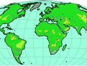
The methane animation (Figure 2) shows where on our planet major methane sources are located and how the strengths of the various sources are changing with time (many of the sources are strongest during the summer months when the biosphere is most active). Important methane sources are wetlands (e.g., Siberia, and central Africa) , rice paddies (e.g., China and India), and ruminants (e.g., India). A possible new source are living plants which may explain the high methane measured by SCIAMACHY over the tropical rain forests. Methane is typically higher over the northern hemisphere compared to the southern hemisphere because most of the sources are located over the northern hemisphere.
Figure 1: CO2 animation: The time dependent spatial distribution of atmospheric CO2 between January 2003 and December 2005 as measured by the SCIAMACHY satellite instrument onboard ENVISAT.
http://www.iup.uni-bremen.de/sciamachy/NIR_NADIR_WFM_DOAS/scia_co2_ani_buchwitz.gif
(Source: SCIAMACHY)
Figure 2: Methane animation: The time dependent spatial distribution of atmospheric methane between January 2003 and December 2005 as measured by the SCIAMACHY satellite instrument onboard ENVISAT.
http://www.iup.uni-bremen.de/sciamachy/NIR_NADIR_WFM_DOAS/scia_ch4_ani_buchwitz.gif
(Source: SCIAMACHY)
Further Reading
- Bergamaschi, P., C. Frankenberg, J. F. Meirink, M. Krol, F. Dentener, T. Wagner, U. Platt, J. O. Kaplan, S. Körner, M. Heimann, E. J. Dlugokencky, and A. Goede, 2007. Satellite chartography of atmospheric methane from SCIAMACHY on board ENVISAT: Evaluation based on inverse model simulations, J. Geophys. Res., 112, D02304, doi:10.1029/2006JD007268.
- Buchwitz, M., R. de Beek, S. Noël, J. P. Burrows, H. Bovensmann, O. Schneising, I. Khlystova, M. Bruns, H. Bremer, P. Bergamaschi, S. Körner, M. Heimann, 2006. Atmospheric carbon gases retrieved from SCIAMACHY by WFM-DOAS: version 0.5 CO and CH4 and impact of calibration improvements on CO2 retrieval, Atmos. Chem. Phys., 6, 2727-275.
- Buchwitz, M., O. Schneising, J. P. Burrows, H. Bovensmann, J. Notholt, 2007. First direct observation of the atmospheric CO2 year-to-year increase from space, Atmos. Chem. Phys. Discuss., 7, 6719-6735.
- ESA, 2007. First greenhouse gas animations produced using Envisat SCIAMACHY data. European Space Agency News, March 20, 2007.
- European environmental satellite ENVISAT.
- Frankenberg, C., J. F. Meirink, M. van Weele, U. Platt, and T. Wagner, 2005. Assessing methane emissions from global space-borne observations, Science, 308, 1010-1014.
- Institute of Environmental Physics / Remote Sensing (iup/ife)
- IPCC, Alley, R., Berntsen, T., Bindoff, N. L., et al., (drafting authors), 2007. Climate change 2007: The physical basis – Summary for policy makers, Contribution of working group I to the Fourth Assessment Report of the Intergovernmental Panel on Climate Change (IPCC), IPCC web page.
- Japanese Greenhouse Gases Observing Satellite (GOSAT)
- Keppler, F., J. T. G. Hamilton, M. Braß, and T. Röckmann, 2006. Methane emissions from terrestrial plants under aerobic conditions, Nature, 439, 187-191.
- NASA's Orbiting Carbon Observatory (OCO)
- NOAA Earth System Research Laboratory.
- SCIAMACHY, 2007. Scanning Imaging Absorption Spectrometer for Atmospheric Chartography