Physical factors mediating ecological change in the Artic

Published: February 9, 2010, 3:29 am

Updated: May 7, 2012, 5:33 pm

Author: International Arctic Science Committee

Topic Editor: Mark McGinley

Topics:

Marine Ecology (main)

Ecology (main)

Climate Change (main)

This is Section 9.3.2 of the Arctic Climate Impact Assessment
Lead Author: Harald Loeng; Contributing Authors: Keith Brander, Eddy Carmack, Stanislav Denisenko, Ken Drinkwater, Bogi Hansen, Kit Kovacs, Pat Livingston, Fiona McLaughlin, Egil Sakshaug; Consulting Authors: Richard Bellerby, Howard Browman,Tore Furevik, Jacqueline M. Grebmeier, Eystein Jansen, Steingrimur Jónsson, Lis Lindal Jørgensen, Svend-Aage Malmberg, Svein Østerhus, Geir Ottersen, Koji Shimada

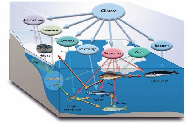
There are a variety of means by which climate can affect marine biota. These can be direct or indirect. Examples of the former include temperature, which affects the metabolism and distribution of organisms; wind-driven currents, which transport planktonic organisms; sea ice (Sea ice in the Arctic), which provides higher predators with a platform for birthing or foraging; and snow (Snow cover in the Arctic), which allows for the construction of overwintering lairs. An indirect means by which climate can affect biota is through those climate processes that affect nutrient levels and surface mixed layer depth, which in turn influence primary and secondary productivity, and ultimately food availability to the upper trophic levels. Figure 9.22 illustrates those climatic factors that can influence the Barents Sea ecosystem, both directly and indirectly. Similar interactions are also valid for other marine areas. The timing of sea-ice formation and melt-back, as well as temperature, can influence the timing, location, and intensity of biological production.

Fig. 9.22. Those climate parameters that may impact upon the marine food chain, both directly and indirectly^[1].

Of the main factors mediating ecological change in the Arctic, the distribution of sea ice (Sea ice effect on marine systems in the Arctic) is most important. Sea ice, together with its snow cover, can reduce light levels at the water surface to those observed at 40 m or more in an ice-free water column. Primary production in the water column below the sea ice is thus severely light-limited. However, the sea ice is of major importance as a habitat for marine mammals and the location of ice edges is extremely important to seabirds. Moreover, the melting of sea ice in spring results in a stratification of the upper water column that promotes primary production.

The flow of warm water into the Arctic and the mixing and stratification of the water column are also important. The flow of warm water into the Arctic is important for the northward transport of zooplankton populations, such as the transport of Calanus finmarchicus from the Norwegian Sea to the Barents Sea. The mixing and stratification of the water column is determined by the opposing forces of wind and freshwater supply^[2].

Generally, sea surface temperatures in the Arctic are low, but true ectotherms (previously called "cold-blooded organisms", i.e., their body temperatures vary with the temperature of their surroundings) can grow at the freezing point of seawater. In principle, organisms grow faster the higher the temperature up to an optimum range, which can be from 8 to 15° C for species living in the Arctic. A temperature increase of 10° C would roughly double the biochemical rates, and thus the growth rate.

The effect of temperature on primary production is largely indirect, through its effect on sea-ice cover and the mixing characteristics of the water column. The direct effect of rising temperature, through its effect on growth rate, would primarily shorten the spring bloom by two to five days, and perhaps slightly increase regenerative production. New production would be likely to increase because it is primarily regulated by the vertical nutrient supply.

Limiting factors

Potentially limiting nutrients in the Arctic are nitrogen or phosphorus, and for diatoms, also silicate. Iron controls primary production by retarding nitrate uptake in the Northeast Pacific and the deep regions of the eastern Bering Sea^[3]. It has also been observed to limit temporarily spring bloom production in the Trondheims fjord^[4]. Silicate, which like nitrogen is also affected by iron control, limits diatom growth in some areas of the Barents Sea^[5]. Because arctic rivers are rich in nitrogen and silicate but poor in phosphate, phosphorus limitation is likely in and around some estuaries.

Most microalgae are probably not limited by CO₂ because they contain the enzyme carbonic acid anhydrase, which can furnish CO₂ from bicarbonate^[6]. Production of the coccoliths that cover coccolithophorids also furnishes CO₂.

In nature, an increase in the supply of the limiting nutrient typically causes a predominance of large-celled species. A sufficient supply of iron and silicate favors large bloom-forming diatoms that enhance the sedimentation rate.

Table 9.7. Winter nutrient levels (mmol/m³) in the Barents Sea, the Bering Sea (surface and at depths >300 m), and the Southern cean (the Ross and Scotia Seas)^[7].
	Barents Sea (Atlantic Water)	Bering Sea (surface water)	Bering Sea (deep water)	Ross Sea (surface water)	Scotia Sea (surface water)
Nitrate	10–12	10–30	45	25	30
Phosphate	0.85	1.0–2.0	3.5	2	2
Silicate	6–8	25–60	100–300	50–60	100

Nutrient status in winter differs strongly between arctic regions, reflecting the nutrient concentration of the deep or intermediate waters that supply nutrients to the upper layers. This is related to the increasing age of the intermediate and deep waters along their THC route. Thus, Atlantic water (which is relatively young) exhibits the lowest concentrations and the deep Bering Sea water (which is older) the highest (Table 9.7). However, because mixing between surface and intermediate water in the Bering Sea is low owing to the high stability of the water column, surface water concentrations in the Bering Sea are actually lower than in the Southern Ocean.

Owing to the high winter nutrient concentrations on the Bering Shelf and in the southern Chukchi Sea, productivity in these regions can be two to four times higher than in the Barents Sea^[8]. Because of its distance from shelf-break upwelling, however, the northeast coastal Alaskan Shelf exhibits low nutrient levels, on a par with those of the Atlantic sector^[9].

North of 85°N, severe light limitation restricts primary production in the water column to a six-week growth season, which is initiated by the melting of the snow on top of the sea ice in July^[10]. In multi-year ice, the dense biomass on the underside of the sea ice is also strongly light-limited, but in melt ponds, intense small-scale production can occur^[11]. Productivity in the multi-year ice in the shelf seas is an order of magnitude greater than in first-year ice, presumably because of a greater nutrient supply, however, the latter generally has very low levels of primary production^[12]. In polynyas, early melting of sea ice can prolong the growth season by three months^[13].

Timing

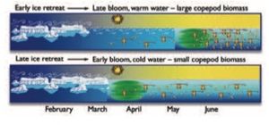
Fig. 9.23. The relative timing of the sea-ice retreat and the spring bloom in the Bering Sea^[14].

In seasonally ice-covered areas, the onset of the phytoplankton bloom is usually determined by the timing of the breakup of the sea ice^[15]. Typically, an ice-edge bloom unfolds in a 20 to 100 km wide belt south of the northward-retreating ice edge. The bloom develops rapidly because water from the melting sea ice establishes a shallow wind-mixed layer of 15 to 35 m depth. The ice-edge bloom generally begins in mid-April to early May at the southernmost fringes of the first-year ice, both in the Barents and Bering Seas and in the Labrador/Newfoundland region^[16]. In the Bering Sea, years with early sea-ice retreat (i.e., starting in winter) have delayed blooms as the blooms cannot begin until light levels and stratification are sufficient to support them. Thus, in the Bering Sea, early ice retreat implies a late bloom, while late ice retreat implies an early bloom (Fig. 9.23). In the Barents Sea, however, very cold winters that result in a more southern distribution of the ice edge (with sea ice forming over Atlantic water to the south of the Polar Front) can have very early blooms because once melting starts the sea ice melts rapidly from below. Near multi-year ice in the Arctic Ocean, melting is delayed until July, resulting in a short growing season^[17], and in the ice-filled regions of the Greenland Sea, late melting can delay the ice-edge bloom until late May as far south as the Denmark Strait^[18].

Impact of physical and chemical forcing

After the ice-edge bloom, primary production becomes very low in the strongly stratified waters, with nutrients near the limit of detection^[19]. In iron-controlled waters, however, there are still high nitrate (Nitrogen) concentrations in the water column. Near the pycnocline (i.e., the region of strongest vertical density gradient) in arctic waters, a restricted vertical supply of nutrients enables the development of a 3 to 10 m thick chlorophyll maximum layer that is strongly light-limited^[20].

In ice-free waters, it is the onset of thermally-derived stratification that determines the timing of the spring bloom. The blooms deplete the upper layer nutrient concentrations. In the Norwegian Sea and the Atlantic (southwest) part of the Barents Sea, thermally-derived water-column stability is established in late May to early June^[21]. In ice-free estuaries and fjords, and waters surrounding Iceland, freshwater-induced stability triggers a bloom in late March to late April^[22]. On continental shelves, nutrient supplies from upwelling or strong tidal mixing can maintain high levels of production, as observed in both the Barents and Bering Seas.

Pulsed (wind-driven) nutrient supplies associated with passing atmospheric low pressure systems often result in small blooms, however, in arctic waters, the pycnocline is usually too strong to allow a temporary deepening of the surface mixed layer and so bring in nutrients from sub-pycnocline waters^[23]. In the Bering Sea, storms, especially those in mid- to late May, lead to a large nutrient supply and prolonged primary production, whereas a weakening of the summer winds lowers the nutrient supply for continuing summer blooms^[24].

Wind-driven nutrient supply supports about 50% of the annual primary production in the southern Barents Sea influenced by the Atlantic inflow and this supply exhibits no clear temporal trend. In the northern Barents Sea, however, primary production clearly follows variations in the NAO index, being high following NAO⁺ years –which correspond to years with relatively warm winters and little sea ice^[25]. The higher production is a result of the reduced sea-ice cover allowing a larger area of the northern Barents Sea exposure to the strong light levels.

For the outer and mid-shelf domains of the Bering Shelf, the wind-driven nutrient supply supports 30 to 50% of the annual primary production, depending on the frequency and intensity of summer storms. Interdecadal trends in chlorophyll-a (Chl-a) concentration were observed by Sugimoto and Tadokoro^[26] in eastern Bering Sea regions deeper than 150 m but it is not known if these resulted in changes in either the spring or overall annual primary production levels. The few available data suggest that the summer contribution to annual new production may have decreased in recent years with the advent of calmer, sunnier summers. Coastal domain production is not thought to vary much between years. On the northern shelf, variability in phytoplankton biomass and production has been linked to variability in the transport of the Bering Slope Current that leads to the Anadyr Stream^[27].

Distribution of primary production

Table 9.8. Estimated levels of primary production, defined as the integrated net photosynthesis (corrected for respiration) over at east 24 hours, plus the grazing rate of mesozooplankton (compiled by Sakshaug^[28] on the basis of data from several authors).
	Area (10³ km²)	Total primary production (g C/m²)	New primary production (g C/m²)	Grazing rate of zooplankton (g C/m²)	Total primary production (Tg C)
Central Deep Arctic	4489	>11	<1	-	>50
Arctic shelves	5052	32	8	10	279
Barents Sea	1512	<20 –200^a	<8–100	15 – 50	136
Barents north slope	-	35	16	-	-
White Sea	90	25	6	-	2
Kara Sea	926	30 –50	7–12	-	37
Laptev Sea	498	25 –40	6–10	-	16
East Siberian Sea	987	25 –40	6–10	-	30
Chukchi Sea	620	20 –>400	5–>160	7 –>90	42
Beaufort Sea	178	30 –70	7–17	-	8
Lincoln Sea	64	20–40	5–10	-	3
Other (Canadian Arctic)	182	20 –40	5–10	-	5
Northeast Water Polynya	<50	20 –50	13–32	-	-
North Water Polynya	-	150	70	-	-
Total Arctic Ocean	9541	>26	<5	-	>329
Atlantic sector	5000	97	50	-	483
Baffin Bay	690	60 –120	25–50	-	62
Hudson Bay	820	50 –70	25–35	-	49
Greenland Sea	600	70	40	-	42
Labrador Sea	1090	100	45	-	110
Norwegian Sea	1400	80 –150	35–65	-	160
Icelandic Sea	400	100 –200^b	45–90	-	60
West Spitsbergen	-	120	55	-	-
Bering Shelf	1300	>230	-	-	>300
Alaskan coastal	-	50 –75	<20	32 –50	-
Siberian coastal	-	>400	>160	>90	-
Middle, outer shelf	-	150 –175	30–50	35 –70	-
Shelf Break	-	450 –900	170–360	-	-
Bering oceanic	1000	60 –180	-	-	155
Okhotsk Sea	1600	100 –200	-	-	240
Global, ocean	362000	110	-	-	40000^c
Global, land	148000	405	-	-	60000
^aHighest values occur where topography and currents cause continuous nutrient supply in Atlantic sector, lowest values in northernmost part; ^bproduction to the south and east of Iceland (i.e., in Atlantic water) is four times that to the north and east; ^cplus 5,000 Tg benthic (seaweed) carbon production and 4,000 to 7,000 Tg of dissolved organic carbon.

The distribution of primary production in the Arctic provides a good illustration of the effects of physical and chemical forcing (Table 9.8). Annual primary production in the deep Arctic Ocean, the lowest known for any sea, reflects the high incidence of multi-year sea ice with snow, and thus the short growing season^[29]. Nevertheless, present estimates are far higher than the pre-1990 estimates, which ignored production within the multi-year ice.

Due to the inflow of Atlantic and Bering Sea water, the Barents Sea and a patch of the Chukchi Sea, respectively, have enhanced annual production^[30] In the other Siberian shelf areas, annual production is low due to multi-year ice hindering wind-driven upwelling of nutrient-rich deep water along the shelf break, leaving re-mixing of nutrient-poor shelf water and phosphorus-poor river water as the main nutrient sources.

In Atlantic water, annual primary production is high, in part due to wind-driven episodic upwelling in summer^[31] (Fig. 9.24). The most productive area is the Bering Shelf where a highly productive "greenbelt" is associated with the upwelling of extremely nutrient-rich water along the shelf break and the Anadyr Current^[32]. In the deep eastern Bering Sea, annual primary productivity is similar to, or slightly higher than that in the Barents Sea^[33].

Secondary production (9.3.2.2)

Although the zooplankton database is small, it suggests that growth rates of calanoid copepods and other crustaceans are dependent on temperature such that the time from hatching to the next adult generation is shorter in warmer water. The growth rate, however, is also very dependent on food supply. More specifically, the growth rate depends on the extent to which the fat-storage organs of the zooplankton are filled to capacity, which in turn is highly dependent on phytoplankton availability^[34]. Nauplii (early-stage larvae) and early-stage copepodite stages can be food-limited at <0.5 to 0.7 mg Chl-a/m³^[35]. This level of concentration is common in waters which receive a low supply of new nutrients due to strong stratification and are therefore dominated by low levels of regenerative primary production^[36].

Match versus mismatch

The concept of match and mismatch is very important in food-web energy transfer. A match implies that the predators are located in the same space and time as their prey and a mismatch when they are not. In principle, grazing by zooplankton is efficient when a large and growing population of zooplankton coincides with a phytoplankton bloom. Production of mesozooplankton is small in areas characterized by a mismatch. This is a highly nonlinear event because phytoplankton blooms and zooplankton swarms are episodic. To ensure a match higher in the food web, fish and zooplankton populations also need to coincide in time and space. Physical oceanographic conditions, such as temperature, salinity, stratification, mixing, and currents can influence the timing and location of the plankton production and biomass as well as the eggs and larvae of fish and invertebrates. In this sense, oceanographic conditions play a large role in determining the extent of a match or mismatch between trophic levels.

Non-grazed phytoplankton sink except for most of the (nanoplankton) fraction that is based on regenerated nutrients. Thus, sedimentation rates are lower when there is a match between phytoplankton and zooplankton. Grazing and sedimentation are thus competing processes and both are strongly dependent on large-celled new production.

Fig. 9.24. Estimated (a) primary production and (b) wind speed for the Atlantic water of the Barents Sea in summer 1998 (wind data and hind-cast model data from the Norwegian meteorological Institute; production model by D. Slagstad, Norwegian University of Science and Technology).^[37].

In Atlantic water, late development of copepodite stages of Calanus finmarchicus is a good match with the late and relatively long-lasting phytoplankton blooms that occur in mid-May to June^[38]. But it is mismatched with the timing of the initial blooms, which is presumably one of the main reasons why C. finmarchicus is allochthonous in the Barents Sea^[39]. The mismatch is greatest in very cold winters when sea ice covers Atlantic water and the blooms are typically four to six weeks earlier than usual^[40]. The reason that the blooms are earlier than usual in such winters is because once melting starts the sea ice over the Atlantic water melts rapidly from below. This can result in the phytoplankton bloom being too early for the zooplankton, thus causing a mismatch in timing with the peak in zooplankton^[41]. Such years can have very low levels of secondary production. Although not strongly correlated, a match seems likely to occur in Atlantic water with mixing depths greater than 40 m, while a mismatch seems likely with mixing depths less than 40 m.

In the generally ice-free Norwegian fjords, the major phytoplankton blooms occur from February to early April, depending on latitude and the extent of Freshwater discharge in the Arcticfreshwater-induced stability. As the major zooplankton peak does not occur until April or May, the zooplankton must feed on the secondary summer and autumn blooms^[42]. Owing to the extreme mismatch, almost all of the early spring bloom sinks to the bottom of the fjord.

Fish (9.3.2.3)

Climate fluctuations affect fish directly, as well as by causing changes in their biological environment (i.e., in relation to predators, prey, species interactions, and disease). Direct physiological effects include changes in metabolic and reproductive processes. Climate variability may influence fish population abundance, principally through effects on recruitment. Variability in the physical environment may also affect feeding rates and competition by favoring one species relative to another, as well as by causing changes in the abundance, quality, size, timing, spatial distribution, and concentration of prey. Variability in the physical environment also affects predation through influences on the abundance and distribution of predators. Fish diseases leading to a weakened state or even death may also be environmentally triggered. Particular temperature ranges may, for instance, be more conducive to allowing disease outbreaks. While water temperature is typically the main source of environmental impact on fish, salinity and oxygen conditions, and ocean mixing and transport processes are also important.

Reproduction, recruitment, and growth

The physical environment affects the reproductive cycle of fish. For example, ambient [[temperature]s] may determine the age at sexual maturity. Atlantic cod off Labrador and the northern Grand Banks mature at 7 yr, while in the warmer waters off southwest Nova Scotia and on Georges Bank they mature at 3.5 and 2 yr, respectively^[43]. Reproduction is typically temperature-dependent with gonad development occurring more quickly under warm conditions. Thus, temperature determines the time of spawning. Examples of low temperatures resulting in delayed spawning have been observed off Newfoundland, both in capelin^[44] and Atlantic cod^[45].

Understanding variability in recruitment (the number of young surviving long enough to potentially enter the fishery) has long been a prime issue in fisheries science. Evidence of changes in fish abundance in the absence of fishing suggests environmental causes. Following spawning, cod eggs and later young stages are generally distributed within the upper water column before they settle toward the bottom as half-year olds. The strength of a year-class is to a large degree determined during the first six months of life^[46]; life stages during which ocean climate may have a decisive effect^[47]. The effects of temperature on recruitment of Atlantic cod across its entire distribution range were examined by Ottersen^[48] and Planque and Fredou^[49]. Populations inhabiting areas at the lower end of the overall temperature range of the species (i.e.,West Greenland, Labrador, Newfoundland, and the Barents Sea) had higher than average recruitment when temperature anomalies were positive, while recruitment to populations occupying the warmer areas (e.g., the Irish and North Seas) seemed better with negative temperature anomalies. For populations inhabiting regions with midrange temperatures the results were inconclusive. The recruitment of Norwegian spring-spawning herring is also linked to variability in water temperature^[50] (see Section 9.3.3.3 (Physical factors mediating ecological change in the Artic)).

The pelagic ecosystem in the southeastern Bering Sea may, according to the recently published Oscillating Control Hypothesis, alternate between primarily bottom:up control in cold regimes and primarily top-down control in warm regimes^[51]. The timing of spring primary production in the southeastern Bering Sea is determined predominately by the timing of sea-ice retreat. Late retreat leads to an early, ice-associated bloom in cold water, whereas no ice, or early retreat, leads to an open-water bloom in warm water. In years when the spring bloom occurs in cold water, low temperatures limit the production of zooplankton, and the survival of larval and juvenile fish, and their recruitment into the populations of large piscivorous fish, such as walleye pollock, Pacific cod, and arrowtooth flounder. Continued over decadal scales, this will lead to bottom:up limitation and a decreased biomass of piscivorous fish. Alternatively, in periods when the bloom occurs in warm water, zooplankton populations should grow rapidly, providing plentiful prey for larval and juvenile fish. Abundant zooplankton will support strong recruitment of fish and will lead to abundant predatory fish that control forage fish, including in the case of walleye pollock, their own juveniles^[52].

Because fish are ectothermic, temperature is the key environmental factor. Individual growth is the result of a series of physiological processes (i.e., feeding, assimilation, metabolism, transformation, and excretion) whose rates are all controlled by temperature^[53]. Brander^[54] examined 17 North Atlantic cod populations and showed that mean bottom temperature accounted for 90% of the observed (ten-fold) difference in growth rates between populations. Higher temperatures led to faster growth rates over the temperature range experienced by these populations. Growth rate decreases at higher temperatures and the temperature for maximum growth decreases as a function of size^[55].

The biomass of zooplankton, the main food for larval and juvenile fish, is generally greater when temperature is high in the Norwegian and Barents Seas^[56]. High food availability for the young fish results in higher growth rates and greater survival through the vulnerable stages that determine year-class strength. Temperature also affects the development rate of fish larvae directly and, thus, the duration of the high-mortality and vulnerable stages decreases with higher temperature^[57]. Also, in the Barents Sea, mean body size as half-year olds fluctuates in synchrony for herring, haddock, and Northeast Arctic cod and the length of all three is positively correlated with water temperature. This indicates that these species, having similar spawning and nursery grounds, respond in a similar manner to large-scale climate fluctuations^[58]. For Barents Sea cod, mean lengths-at-age for ages 1 to 7 are greater in warm periods^[59].

For 2- and 3-year old Barents Sea capelin, Gjøsæter and Loeng^[60] found positive correlations between temperature and growth for different geographical regions and for different years. Changes in water temperature through altered climate patterns may also affect predator–prey interactions. In the Barents Sea, the increase in basic metabolic rates of Northeast Arctic cod, associated with higher temperatures, can result in a rise in the consumption of capelin by 100,000 tonnes per degree centigrade^[61].

Distribution and migration

Temperature is one of the main factors, together with food availability and suitable spawning grounds, which determines the large-scale distribution pattern of fish. Because most fish species (and stocks) tend to prefer a specific temperature range^[62], long-term changes in temperature can lead to expansion or contraction of the distribution range of a species. These changes are generally most evident near the northern or southern boundaries of the species range; warming results in a northward shift and cooling draws species southward. For example, in the Barents Sea, temperature-related displacement of Northeast Arctic cod has been reported on inter-annual time scales as well as at both small and large spatial scales. In warm periods, cod distribution is extended eastward and northward compared to colder periods when the fish tend to concentrate in the southwestern part of the Barents Sea^[63]. Capelin distribution also responds to changes in water temperature both in the Barents Sea^[64] and off Newfoundland and Labrador.

The relatively high interannual stability of residual currents, which prevail in most regions, maintains the main features of larval drift patterns from spawning area to bottom settlement area for each population, and consolidates differences between populations. Interannual variation is introduced through changes in large-and-regional-scale atmospheric pressure conditions. These affect [[wind]s] and upper ocean currents, which in turn modify drift patterns of fish larvae and introduce variability in water temperature and the availability of prey items. While a long and unrestricted larval drift is important for some cod populations, such as those in the Barents Sea and the Icelandic component at West Greenland, recruitment to populations residing in small and open systems depends on larval retainment and the avoidance of massive advective losses^[65].

Many species that undertake seasonal migrations appear to use environmental conditions as cues. For example, April sea surface temperatures and sea-ice (Sea ice in the Arctic) conditions in the southern Gulf of St. Lawrence determine the average arrival time of Atlantic herring on their spawning grounds^[66]. Sea-ice conditions also appear to control the arrival time in spring of Atlantic cod onto the Magdalen Shallows into the Gulf of St. Lawrence^[67]. Atlantic salmon arrive earlier along the Newfoundland and Labrador coasts during warmer years^[68].

The Norwegian spring-spawning herring stock, inhabiting the Norwegian and Icelandic Seas, is highly migratory. Larvae and fry drift into the Barents Sea, while adults undergo substantial feeding and spawning migrations^[69]. Since around 1950, biomass and migration patterns have fluctuated dramatically. While these shifting migration patterns may be dominated by density-dependence, environmental conditions are also likely to have been important^[70].

In the Bering Sea, warmer bottom [[temperature]s] lead to the distribution of adult walleye pollock, Greenland turbot, yellow Irish lord (Hemilepidotus jordani), and thorny sculpin (Icelus spiniger) being more widespread on the shelf, while Arctic cod are restricted to the cold pool^[71].

The combination of environmentally influenced distribution patterns and politically restricted fisheries patterns can have pronounced impacts on the availability of fish to fishers. For instance, most of the Barents Sea is under either Norwegian or Russian jurisdiction, but there is a small, disputed region of international waters in the center. This area is aptly named the "Loophole" and at times it is the site of extensive fishing activity by the international fishing fleets. Most fishing occurs in the southern part of the Loophole, where in warmer years several species of all sizes are found throughout the year. However, in colder years there may be hardly any fish in the area for prolonged periods. The reason for this pattern is that the southern part of the Loophole lies to the south of the Polar Front so that even relatively small east–west movements of the water masses may result in large temperature changes. In cold years, the Polar Front is displaced farther south and west than the Loophole. The fish move in order to remain within the warmer water, thereby making them unavailable to the international fishing fleets^[72]. The movement of the Polar Front is most pronounced between warm and cold years in the Barents Sea as a whole, but movements may also occur on time scales of weeks.

Marine mammals and seabirds (9.3.2.4)

Some important predator–prey match–mismatch issues also occur with higher predators. The timing of reproduction in many seal species is thought to match the availability of large zooplankton and small fishes at the time when pups are weaned and when polar bear den emergence occurs during the peak reproductive period of their favorite prey, ringed seal. Likewise, invertebrate or fish species must be available in the upper parts of the water column when seabird young commence self-feeding. Higher predators might not easily track shifts in the production of zooplankton and fish, which are more directly influenced by temperature.

Factors that influence the distribution and annual duration of sea ice (Sea ice in the Arctic) or snow (Snow cover in the Arctic) availability in the spring can potentially have profound influences on the population ecology of some arctic marine mammals. Sea ice is the breeding habitat for all pagophilic (i.e., ice-loving) seal species and it is the primary hunting platform for polar bear. Changes in the time of formation or disappearance of seasonal sea ice, in the quality of the sea ice, and in the extent of total coverage of both seasonal and multi-year ice could all affect ice-dependent species. Snow cover is very important for polar bears and ringed seals and changes in average snow depth or duration of the snow season could affect their breeding success.

Walruses appear to follow an annual migratory pattern, moving with the advance and retreat of the sea ice in most parts of their range^[73]. However, this may be due to the sea ice blocking access to shallow-water feeding areas, rather than to it serving as an essential habitat element.

The primary requirement for seabirds in the Arctic is suitable breeding cliffs near abundant prey sources. If ice edges or frontal regions shift such that the distance between these highly productive areas and the nesting areas becomes too great, the mismatch would have serious consequences for seabirds.

Chapter 9: Marine Systems
9.1. Introduction (Physical factors mediating ecological change in the Artic)
9.2. Physical oceanography
9.2.1. General features (Physical factors mediating ecological change in the Artic)
9.2.2. Sea ice (Sea ice effect on marine systems in the Arctic)
9.2.3. Ocean processes of climatic importance
9.2.4. Variability in hydrographic properties and currents
9.2.5. Anticipated changes in physical conditions
9.3. Biota
9.3.1. General description of the Arctic biota community
9.3.2. Physical factors mediating ecological change
9.3.3. Past variability – interannual to decadal
9.3.4. Future change – processes and impacts on biota
9.4. Effects of changes in ultraviolet radiation
9.5. The carbon cycle and climate change
9.6. Key findings (Physical factors mediating ecological change in the Artic)
9.7. Gaps in knowledge and research needs

References

Citation

Committee, I. (2012). Physical factors mediating ecological change in the Artic. Retrieved from http://editors.eol.org/eoearth/wiki/Physical_factors_mediating_ecological_change_in_the_Artic

↑ Stenseth, N.C., A. Mysterud, G. Ottersen, J.W. Hurrell, K.-S. Chan and M. Lima, 2002. Ecological effects of climate fluctuations. Science, 297:1292–1296.
↑ Sakshaug, E. and D. Slagstad, 1992. Sea ice and wind: Effects on primary productivity in the Barents Sea. Atmosphere-Ocean, 30:579–591.
↑ Frost, B.W. and M.J. Kishi, 1999. Ecosystem dynamics in the eastern and western gyres of the subarctic Pacific – a review of lower trophic level modelling. Progress in Oceanography, 43:317–333.
↑ Öztürk, M., E. Steinnes and E. Sakshaug, 2002. Iron speciation in the Trondheim Fjord from the perspective of iron limitation for phytoplankton. Estuarine Coastal and Shelf Science, 55:197–212.
↑ Nielsen, T.G. and B. Hansen, 1995. Plankton community structure and carbon cycling on the western coast of Greenland during and after the sedimentation of a diatom bloom. Marine Ecology Progress Series, 125:239–257.–Wassmann, P., T. Ratkova, I. Andreassen, M. Vernet, C. Pedersen and F. Rey, 1999. Spring bloom development in the marginal ice zone and the Central Barents Sea. Pubblicazioni della Stazione Zoologica di Napoli I: Marine Ecology, 20:321–346.
↑ Anning, T., N. Nimer, M.J. Merrett and C. Brownlee, 1996. Costs and benefits of calcification in coccolithophorids. Journal of Marine Systems, 9:45–56.–Goldman, J.C., 1999. Inorganic carbon availability and the growth of large marine diatoms. Marine Ecology Progress Series, 180:81–91.–Reinfelder, J.R., A.M.L. Kraepiel and F.M.M. Morel, 2000. Unicellular C4 photosynthesis in a marine diatom. Nature, 407:996–999.–Sültemeyer, D., 1998. Carbonic anhydrase in eukaryotic algae: characterization, regulation, and possible function during photosynthesis. Canadian Journal of Botany, 76:962–972.
↑ Sakshaug, E., 2003. Primary and secondary production in Arctic Seas. In: R. Stein and R.W. Macdonald (eds.). The Organic Carbon Cycle in the Arctic Ocean, pp. 57–81. Springer, Berlin.
↑ Coachman, L.K., T.E. Whitledge and J.J. Goering, 1999. Silica in Bering Sea deep and bottom water. In: T.R. Loughlin and K. Ohtani (eds.). Dynamics of the Bering Sea, pp. 285–310. University of Alaska Fairbanks.–Grahl, C., A. Boetius and E.M. Nöthig, 1999. Pelagic-benthic coupling in the Laptev Sea affected by ice cover. In: H. Kassens, H.A. Bauch, I.A. Dmitrenko, H. Eicken, H.-W. Hubberten, M. Melles, J. Thiede and L.A. Timokhov (eds.). Land-Ocean Systems in the Siberian Arctic: Dynamics and History, pp. 143–152. Springer, Berlin.–Olsen, A., T. Johannessen and F. Rey, 2003. On the nature of the factors that control spring bloom development at the entrance to the Barents Sea and their interannual variability. Sarsia, 88(6):379–393.–Schlosser, P., J.L. Bullister, R. Fine, W.J. Jenkins, R. Key, J. Lupton, W. Roether and W.M. Smethie Jr., 2001. Transformation and age of water masses. In: G. Siedler, J. Church and J. Gould (eds.). Ocean Circulation and Climate; Observing and Modelling the Global Ocean, pp. 431–452. Academic Press.–Shiomoto, A., 1999. Effect of nutrients on phytoplankton size in the Bering Sea Basin. In: T.R. Loughlin and K. Ohtani (eds.). Dynamics of the Bering Sea, pp. 323–340. University of Alaska Fairbanks.–Walsh, J.J. and D.A. Dieterle, 1994. CO2 cycling in the coastal ocean. I. A numerical analysis of the southeastern Bering Sea with applications to the Chukchi Sea and the northern Gulf of Mexico. Progress in Oceanography, 34:335–392.
↑ Coachman, L.K. and J.J. Walsh, 1981. A diffusion model of cross-shelf exchange of nutrients in the southeastern Bering Sea. Deep-Sea Research A, 28:819–846.
↑ English, T.S., 1961. Some biological observations in the central North Polar Sea. Drift Station Alpha 1957–1958. Arctic Institute of North America Research Paper, 13:8–80.–Kawamura, A., 1967. Observations of phytoplankton in the Arctic Ocean in 1964. Bulletin of the Plankton Society of Japan, 1967:71–89.–Usachev, P.I., 1961. Phytoplankton of the North Pole. Fisheries Research Board of Canada Translation Series, 1285.
↑ Booth, B.C. and R.A. Horner, 1997. Microalgae on the Arctic Ocean Section, 1994: species abundance and biomass. Deep-Sea Research II, 44:1607–1622.–Gosselin, M., M. Levasseur, P.A. Wheeler, R.A. Horner and B.C. Booth, 1997. New measurements of phytoplankton and ice algal production in the Arctic Ocean. Deep-Sea Research II, 44:1623–1644.–Sherr, E.B., B.F. Sherr and L. Fessenden, 1997. Heterotrophic protists in the Central Arctic Ocean. Deep-Sea Research II, 44:1665–1673.
↑ Andersen, O.G.N., 1989. Primary production, chlorophyll, light, and nutrients beneath the Arctic sea ice. In: Y. Herman (ed.). The Arctic Seas: Climatology, Oceanography, Geology and Biology, pp. 147–191. van Nostrand Reinhold, New York.–Gradinger, R., 1996. Occurrence of an algal bloom under Arctic pack ice. Marine Ecology Progress Series, 131:301–305.–Juterzenka, K.V. and K. Knickmeier, 1999. chlorophyll a in water column and sea ice during the Laptev Sea freeze-up study in autumn 1995. In: H. Kassens, H.A. Bauch, I.A. Dmitrenko, H. Eicken, H.-W. Hubberten, M. Melles, J. Thiede and L.A. Timokhov (eds.). Land-Ocean Systems in the Siberian Arctic: Dynamics and History, pp. 153–160. Springer.
↑ Smith, W.O. Jr., M. Gosselin, L. Legendre, D. Wallace, K. Daly and G. Kattner, 1997. New production in the Northeast Water Polynya: 1993. Journal of Marine Systems, 10:199–209.–Suzuki, Y., S. Kudoh and M. Takahashi, 1997. Photosynthetic and respiratory characteristics of an Arctic ice algal community living in low light and low temperature conditions. Journal of Marine Systems, 11:111–121.
↑ Hunt, G.L. Jr., P. Stabeno, G. Walters, E. Sinclair, R.D. Brodeur, J.M. Napp and N.A. Bond, 2002. Climate change and control of the southeastern Bering Sea pelagic ecosystem. Deep-Sea Research II, 49:5821–5853.
↑ Alexander, V. and H.J. Niebauer, 1981. Oceanography of the eastern Bering Sea ice-edge zone in spring. Limnology and Oceanography, 26:1111–1125.–Braarud, T., 1935. The Øst Expedition to the Denmark Strait in 1929. II. The phytoplankton and its conditions of growth. Hvalradets Skrifter, 10:1–173.–Gran, H.H., 1931. On the conditions for the production of the plankton in the sea. ICES Rapports et Procès-Verbaux des Réunions, 75:37–46.–Head, E.J.H., L.R. Harris and R.W. Campbell, 2000. Investigations on the ecology of Calanus spp. in the Labrador Sea. I. Relationship between the phytoplankton bloom and reproduction and development of Calanus finmarchicus in spring. Marine Ecology Progress Series, 193:53–73.–Stabeno, P.J., N.A. Bond, N.B. Kachel, S.A. Salo and J.D. Schumacher, 2001. On the temporal variability of the physical environment over the south-eastern Bering Sea. Fisheries Oceanography, 10(1):81–98.–Wassmann, P., T. Ratkova, I. Andreassen, M. Vernet, C. Pedersen and F. Rey, 1999. Spring bloom development in the marginal ice zone and the Central Barents Sea. Pubblicazioni della Stazione Zoologica di Napoli I: Marine Ecology, 20:321–346.
↑ Alexander, V. and H.J. Niebauer, 1981. Oceanography of the eastern Bering Sea ice-edge zone in spring. Limnology and Oceanography, 26:1111–1125.
↑ Strass, V.H. and E.-M. Nöthig, 1996. Seasonal shifts in ice edge phytoplankton blooms in the Barents Sea related to the water column stability. Polar Biology, 16:409–422.
↑ Braarud, T., 1935. The Øst Expedition to the Denmark Strait in 1929. II. The phytoplankton and its conditions of growth. Hvalradets Skrifter, 10:1–173.
↑ Fujishima, Y., K. Ueda, M. Maruo, E. Nakayama, C. Tokutome, H. Hasegawa, M. Matsui and Y. Sohrin, 2001. Distribution of trace bioelements in the Subarctic North Pacific Ocean and the Bering Sea (the R/V Hakuho Maru cruise KH-97-2). Journal of Oceanography, 57:261–273.–Taniguchi, A., 1999. Differences in the structure of the lower trophic levels of pelagic ecosystems in the eastern and western subarctic Pacific. Progress in Oceanography, 43:289–315.–Whitledge, T.E. and V.A. Luchin, 1999. Summary of chemical distributions and dynamics in the Bering Sea. In: T.R. Loughlin and K. Ohtani (eds.). Dynamics of the Bering Sea, pp. 217–249. University of Alaska Sea.
↑ Heiskanen, A.-S. and A. Keck, 1996. Distribution and sinking rates of phytoplankton, detritus, and particulate biogenic silica in the Laptev Sea and Lena River (Arctic Siberia). Marine Chemistry, 53:229–245.–Luchetta, A., M. Lipizer and G. Socal, 2000. Temporal evolution of primary production in the central Barents Sea. Journal of Marine Systems, 27:177–193.–Nielsen, T.G. and B. Hansen, 1995. Plankton community structure and carbon cycling on the western coast of Greenland during and after the sedimentation of a diatom bloom. Marine Ecology Progress Series, 125:239–257.
↑ Halldal, P., 1953. Phytoplankton investigations from weather ship M in the Norwegian Sea, 1948–1949. Hvalradets Skrifter, 38:1–91.–Olsen, A., T. Johannessen and F. Rey, 2003. On the nature of the factors that control spring bloom development at the entrance to the Barents Sea and their interannual variability. Sarsia, 88(6):379–393.–Paasche, E., 1960. Phytoplankton distribution in the Norwegian Sea in June, 1954, related to hydrography and compared with primary production data. Fiskeridirektoratets Skrifter, Serie Havundersokelser, 12(2):1–77.–Steemann-Nielsen, E., 1935. The production of phytoplankton at the Faroe Isles, Iceland, East Greenland and in the waters around. Meddelelser fra Kommissionen for Danmarks Fiskeri - Og Havunder Soegelser, 3(1):1–93.
↑ Gislason, A. and O.S. Ástthórsson, 1998. Seasonal variations in biomass, abundance and composition of zooplankton in the subarctic waters north of Iceland. Polar Biology, 20:85–94.–Braarud, T., 1935. The Øst Expedition to the Denmark Strait in 1929. II. The phytoplankton and its conditions of growth. Hvalradets Skrifter, 10:1–173.–Sakshaug, E., 1972. Phytoplankton investigations in Trondheimsfjord, 1963–1966. Det Kongelige Norske Videnskabernes Selskabs Skrifter, 1972(1):1–56.
↑ Overland, J.E., S.A. Salo, L.H. Kantha and A.C. Clayson, 1999b. Thermal stratification and mixing on the Bering Sea shelf. In: T.R. Loughlin and K. Ohtani (eds.). Dynamics of the Bering Sea, pp. 129–146. University of Alaska Fairbanks.–Sakshaug, E. and D. Slagstad, 1992. Sea ice and wind: Effects on primary productivity in the Barents Sea. Atmosphere-Ocean, 30:579–591.
↑ Stabeno, P.J., N.A. Bond, N.B. Kachel, S.A. Salo and J.D. Schumacher, 2001. On the temporal variability of the physical environment over the south-eastern Bering Sea. Fisheries Oceanography, 10(1):81–98.
↑ Slagstad, D. and K. Støle-Hansen, 1991. Dynamics of plankton growth in the Barents Sea: model studies. Polar Research, 10:173–186.
↑ Sugimoto, T. and K. Tadokoro, 1997. Interannual-interdecadal variations in zooplankton biomass, chlorophyll concentration and physical environment in the subarctic Pacific and Bering Sea. Fisheries Oceanography, 6(2):74–93.
↑ Springer, A.M., C. McRoy and M.V. Flint, 1996. The Bering Sea green belt: shelf edge processes and ecosystem production. Fisheries Oceanography, 5:205–223.
↑ Sakshaug, E., 2003. Primary and secondary production in Arctic Seas. In: R. Stein and R.W. Macdonald (eds.). The Organic Carbon Cycle in the Arctic Ocean, pp. 57–81. Springer, Berlin.
↑ Cota, G.F., L.R. Pomeroy, W.G. Harrison, E.P. Jones, F. Peters, W.M. Sheldon Jr. and T.R. Weingartner, 1996. Nutrients, primary production and microbial heterotrophy in the southeastern Chukchi Sea: Arctic summer nutrient depletion and heterotrophy. Marine Ecology Progress Series, 135:247–258.–Gosselin, M., M. Levasseur, P.A. Wheeler, R.A. Horner and B.C. Booth, 1997. New measurements of phytoplankton and ice algal production in the Arctic Ocean. Deep-Sea Research II, 44:1623–1644.
↑ Hegseth, E.N., 1998. Primary production of the northern Barents Sea. Polar Research, 17(2):113–123.–Noji, T., L.A. Miller, I. Skjelvan, E. Falck, K.Y. Børsheim, F. Rey, J. Urban-Rich and T. Johannessen, 2000. Constraints on carbon drawdown and export in the Greenland Sea. In: P. Schäfer, W. Ritzrau, M. Schlüter and J. Thiede (eds.). The Northern North Atlantic: A Changing Environment, pp. 39–52. Springer, Berlin. Norderhaug, M., E. Bruun and G.U. Mollen, 1977. Barentshavet sjofuglressurser. Norsk Polarinstitutt Meddelelser, 104:1–119. (In Norwegian with English summary)–Sakshaug, E. and D. Slagstad, 1992. Sea ice and wind: Effects on primary productivity in the Barents Sea. Atmosphere-Ocean, 30:579–591.–Smith,W.O. Jr., M. Gosselin, L. Legendre, D.Wallace, K. Daly and G. Kattner, 1997. New production in the Northeast Water Polynya: 1993. Journal of Marine Systems, 10:199–209.–Walsh, J.J. and D.A. Dieterle, 1994. CO2 cycling in the coastal ocean. I. A numerical analysis of the southeastern Bering Sea with applications to the Chukchi Sea and the northern Gulf of Mexico. Progress in Oceanography, 34:335–392.
↑ Olsen, A., T. Johannessen and F. Rey, 2003. On the nature of the factors that control spring bloom development at the entrance to the Barents Sea and their interannual variability. Sarsia, 88(6):379–393.–Sakshaug, E. and D. Slagstad, 1992. Sea ice and wind: Effects on primary productivity in the Barents Sea. Atmosphere-Ocean, 30:579–591.
↑ Hansell, D.A., T.E. Whitledge and J.J. Goering, 1993. Patterns of nitrate utilization and new production over the Bering-Chukchi shelf. Continental Shelf Research, 13:601–627.–Nihoul, J.C.J., P. Adam, P. Brasseur, E. Deleersnijder, S. Djenidi and J. Haus, 1993. Three-dimensional general circulation model of the northern Bering Sea's summer ecohydrodynamics. Continental Shelf Research, 13:509–542.–Springer, A.M., C. McRoy and M.V. Flint, 1996. The Bering Sea green belt: shelf edge processes and ecosystem production. Fisheries Oceanography, 5:205–223.–Walsh, J.J., C.P. McRoy, L.K. Coachman, J.J. Goering, J.J. Nihoul, T.E. Whitledge, T.H. Blackburn, P.L. Parker, C.D. Wirick, P.G. Stuert, J.M. Grebmeier, A.M. Springer, R.D. Tripp, D.A. Hansell, S. Djenidi, E. Deleersnijder, K. Henriksen, B.A. Lund, P. Andersen, F.E. Muller-Karger and K. Dean, 1989. Carbon and nitrogen cycling within the Bering/Chukchi Seas: Source regions for organic matter effecting AOU demands of the Arctic Ocean. Progress in Oceanography, 22:277–359.
↑ Maita, Y., M. Yanada and T. Takahashi, 1999. Seasonal variation in the process of marine organism production based on downward fluxes of organic substances in the Bering Sea. In: T.R. Loughlin and K. Ohtani (eds.). Dynamics of the Bering Sea, pp. 341–352. University of Alaska Fairbanks.–Springer, A.M., C. McRoy and M.V. Flint, 1996.The Bering Sea green belt: shelf edge processes and ecosystem production. Fisheries Oceanography, 5:205–223.
↑ Hygum, B.H., C. Rey and B.W. Hansen, 2000. Growth and development rates of Calanus finmarchicus nauplii during a diatom spring bloom. Marine Biology, 136:1075–1085.
↑ Campbell, R.G., J.A. Runge and E.G. Durbin, 2001. Evidence for food limitation of Calanus finmarchicus production rates on the southern flank of Georges Bank during April 1997. Deep-Sea Research II, 48:531–549.
↑ Båmstedt, U., H.C. Eilertsen, K.S. Tande, D. Slagstad and H.R. Skjoldal, 1991. Copepod grazing and its potential impact on the phytoplankton development in the Barents Sea. Polar Research, 10:339–353.–Booth, B.C., J. Lewin and J.R. Postel, 1993. Temporal variation in the structure of autotrophic and heterotrophic communities in the subarctic Pacific. Progress in Oceanography, 32:57–99.–Hirche, H.-J. and S. Kwasniewski, 1997. Distribution, reproduction and development of Calanus species in the Northeast water in relation to environmental conditions. Journal of Marine Systems, 10:299–317.–Irigoien, X., R. Head, U. Klenke, B. Meyer-Harms, D. Harbour, B. Niehoff, H.-J. Hirche and R. Harris, 1998. A high frequency time series at Weathership M, Norwegian Sea, during the 1997 spring bloom: feeding of adult female Calanus finmarchicus. Marine Ecology Progress Series, 172:127–137.
↑ Slagstad, D. pers. comm. Norwegian University of Science and Technology.
↑ Dalpadado, P. and H.R. Skjoldal, 1991. Distribution and life history of krill from the Barents Sea. Polar Research, 10:443–460.–Skjoldal, H.R., A. Hassel, F. Rey and H. Loeng, 1987. Spring phytoplankton development and zooplankton reproduction in the central Barents Sea in the period 1979–84. In: H. Loeng (ed.). Proceedings of the Third Soviet-Norwegian Symposium, Murmansk, 1986, pp. 59–89. Institute of Marine Research, Bergen, Norway.
↑ Melle, W. and H.R. Skjoldal, 1998. Reproduction and development of Calanus finmarchicus, C. glacialis and C. hyperboreus in the Barents Sea. Marine Ecology Progress Series, 169:211–228.
↑ Olsen, A., T. Johannessen and F. Rey, 2003. On the nature of the factors that control spring bloom development at the entrance to the Barents Sea and their interannual variability. Sarsia, 88(6):379–393.
↑ Olsen, A., T. Johannessen and F. Rey, 2003. On the nature of the factors that control spring bloom development at the entrance to the Barents Sea and their interannual variability. Sarsia, 88(6):379–393.–Skjoldal, H.R. and F. Rey, 1989. Pelagic production and variability of the Barents Sea ecosystem. In: K. Sherman and L.M. Alexander (eds.). Biomass Yields and Geography of Large Marine Ecosystems, pp. 241–286. AAAS Selected Symposium 111. Westview Press, Colorado.
↑ Wassmann, P., 1991. Dynamics of primary production and sedimentation in shallow fjords and polls of western Norway. In: H. Barnes, A.D. Ansell and R.N. Gibson (eds.). Oceanography and Marine Biology: An Annual Review, 29:87–154.
↑ Drinkwater, K.F., 1999. Changes in ocean climate and its general effect on fisheries: examples from the North-west Atlantic. In: D. Mills (ed.).The Ocean Life of Atlantic Salmon - Environmental and Biological Factors Influencing Survival, pp. 116–136. Fishing News Books, Oxford.
↑ Nakashima, B.S., 1996. The relationship between oceanographic conditions in the 1990s and changes in spawning behaviour, growth and early life history of capelin (Mallotus villosus). NAFO Scientific Council Studies, 24:55–68.
↑ Hutchings, J.A. and R.A. Myers, 1994. Timing of cod reproduction: interannual variability and the influence of temperature. Marine Ecology Progress Series, 108:21–31.
↑ Helle, K., B. Bogstad, C.T. Marshall, K. Michalsen, G. Ottersen and M. Pennington, 2000. An evaluation of recruitment indices for Arcto-Norwegian cod (Gadus morhua L.). Fisheries Research, 48(1):55–67.–Hjort, J., 1914. Fluctuations in the great fisheries of northern Europe viewed in the light of biological research. ICES Rapports et Procès-Verbaux des Réunions, 20:1–228.–Myers, R.A. and N.G. Cadigan, 1993. Density-dependent juvenile mortality in marine demersal fish. Canadian Journal of Fisheries and Aquatic Sciences, 50:1576–1590.–Sundby, S., H. Bjørke, A.V. Soldal and S. Olsen, 1989. Mortality rates during the early life stages and year class strength of northeast Arctic cod (Gadus morhua L.). ICES Rapports et Procès-Verbaux des Réunions, 191:351–358.
↑ Cushing, D.H., 1966. Biological and hydrographic changes in British Seas during the last thirty years. Biological Reviews, 41:221–258.–De Young, B. and G.A. Rose, 1993. On recruitment and distribution of Atlantic cod (Gadus morhua) off Newfoundland. Canadian Journal of Fisheries and Aquatic Sciences, 50:2729–2741.–Dickson, R.R. and K.M. Brander, 1993. Effects of a changing wind-field on cod stocks of the North Atlantic. Fisheries Oceanography, 2:124–153.–Ellertsen, B., P. Fossum, P. Solemdal and S. Sundby, 1989. Relation between temperature and survival of eggs and first-feeding larvae of northeast Arctic cod (Gadus morhua L.). ICES Rapports et Procès-Verbaux des Réunions, 191:209–219.–Ottersen, G. and S. Sundby, 1995. Effects of temperature, wind and spawning stock biomass on recruitment of Arcto-Norwegian cod. Fisheries Oceanography, 4:278–292.–Sætersdal, G. and H. Loeng, 1987. Ecological adaption of reproduction in Northeast Arctic cod. Fisheries Research, 5:253–270.
↑ Ottersen, G. 1996. Environmental Impact on Variability in Recruitment, Larval Growth and Distribution of Arcto–Norwegian Cod. Geophysical Institute, University of Bergen, 136pp.
↑ Planque, B. and T. Fredou, 1999. Temperature and the recruitment of Atlantic cod (Gadus morhua). Canadian Journal of Fisheries and Aquatic Sciences, 56:2069–2077.
↑ Toresen, R. and O.J. Østvedt, 2000. Variation in abundance of Norwegian spring-spawning herring (Clupea harengus, Clupeidae) throughout the 20th century and the influence of climatic fluctuations. Fish and Fisheries, 1:231–256.
↑ Hunt, G.L. Jr. and P.J. Stabeno, 2002. Climate change and the control of energy flow in the southeastern Bering Sea. Progress in Oceanography, 55:5–22.–Hunt, G.L. Jr., P. Stabeno, G. Walters, E. Sinclair, R.D. Brodeur, J.M. Napp and N.A. Bond, 2002. Climate change and control of the southeastern Bering Sea pelagic ecosystem. Deep-Sea Research II, 49:5821–5853.
↑ Hunt, G.L. Jr. and P.J. Stabeno, 2002. Climate change and the control of energy flow in the southeastern Bering Sea. Progress in Oceanography, 55:5–22.–Hunt, G.L. Jr., P. Stabeno, G. Walters, E. Sinclair, R.D. Brodeur, J.M. Napp and N.A. Bond, 2002. Climate change and control of the southeastern Bering Sea pelagic ecosystem. Deep-Sea Research II, 49:5821–5853.
↑ Brett, J.R., 1979. Environmental factors and growth. In: W.S. Hoar, D.J. Randal and J.R. Brett (eds.). Fish Physiology, vol. 8, pp. 599–675. Academic Press.–Michalsen, K., G. Ottersen and O. Nakken, 1998. Growth of North-east Arctic cod (Gadus morhua L.) in relation to ambient temperature. ICES Journal of Marine Science, 55:863–877.
↑ Brander, K.M., 1994. Patterns of distribution, spawning and growth in North Atlantic cod: the utility of inter-regional comparisons. ICES Marine Science Symposia, 198:406–413.–Brander, K.M., 1995. The effect of temperature on growth of Atlantic cod (Gadus morhua L.). ICES Journal of Marine Science, 52:1–10.
↑ Björnsson, B., A. Steinarsson and M. Oddgeirsson, 2001. Optimal temperature for growth and feed conversion of immature cod (Gadus morhua L.). ICES Journal of Marine Science, 58(1):29–38.
↑ Nesterova, V.N., 1990. Plankton biomass along the drift route of cod larvae. Pinro, Murmansk, 64pp. (In Russian)
↑ Blood, D.M., 2002. Low-temperature incubation of walleye pollock (Theragra chalcogramma) eggs from the southeast Bering Sea shelf and Shelikof Strait, Gulf of Alaska. Deep-Sea Research II, 49:6095–6108.–Coyle, K.O. and A.I. Pinchuk, 2002. Climate-related differences in zooplankton density and growth on the inner shelf of the southeastern Bering Sea. Progress in Oceanography, 55:177–194.–Ottersen, G. and H. Loeng, 2000. Covariability in early growth and year-class strength of Barents Sea cod, haddock and herring: The environmental link. ICES Journal of Marine Science, 57:339–348.–Ottersen, G. and S. Sundby, 1995. Effects of temperature, wind and spawning stock biomass on recruitment of Arcto-Norwegian cod. Fisheries Oceanography, 4:278–292.
↑ Loeng, H., H. Bjørke and G. Ottersen, 1995. Larval fish growth in the Barents Sea. In: R.J. Beamish (ed.). Climate Change and Northern Fish Populations. Canadian Special Publication of Fisheries and Aquatic Sciences, 121:691–698.–Ottersen, G. and H. Loeng, 2000. Covariability in early growth and year-class strength of Barents Sea cod, haddock and herring: The environmental link. ICES Journal of Marine Science, 57:339–348.
↑ Dementyeva, T.F. and E.M. Mankevich, 1965. Changes in growth rate of Barents Sea cod as affected by environmental factors. International Commission for the Northwest Atlantic Fisheries, Special Publication, 6:571–577.–Michalsen, K., G. Ottersen and O. Nakken, 1998. Growth of North-east Arctic cod (Gadus morhua L.) in relation to ambient temperature. ICES Journal of Marine Science, 55:863–877.–Nakken, O. and A. Raknes, 1987. The distribution and growth of Northeast Arctic cod in relation to bottom temperatures in the Barents Sea, 1978–1984. Fisheries Research, 5:243–252.
↑ Gjøsæter, H. and H. Loeng, 1987. Growth of the Barents Sea capelin, Mallotus villosus, in relation to climate. Environmental Biology of Fishes, 20:293–300.
↑ Bogstad, B. and H. Gjøsæter, 1994. A method for estimating the consumption of capelin by cod in the Barents Sea. ICES Journal of Marine Science, 51:273–280.
↑ Coutant, C.C., 1977. Compilation of temperature preference data. Journal of the Fisheries Research Board of Canada, 34:739–745.–Scott, J.S., 1982. Depth, temperature and salinity preferences of common fishes of the Scotian Shelf. Journal of Northwest Atlantic Fishery Science, 3:29–39.
↑ Ottersen, G., K. Michalsen and O. Nakken, 1998. Ambient temperature and distribution of north-east Arctic cod. ICES Journal of Marine Science, 55:67–85.
↑ Sakshaug, E., A. Bjørge, B. Gulliksen, H. Loeng and F. Mehlum (eds.), 1992. Okosystem Barentshavet. Universitetsforlaget (2. utgivelse), Oslo, 304pp.
↑ Ottersen, G. 1996. Environmental Impact on Variability in Recruitment, Larval Growth and Distribution of Arcto–Norwegian Cod. Geophysical Institute, University of Bergen, 136pp.–Sinclair, M., 1988. Marine Populations: An Essay on Population Regulation and Speciation. University of Washington Press, Seattle, 252pp.
↑ Lauzier, L.M. and S.N. Tibbo, 1965. Water temperature and the herring fishery of Magdalen Islands, Quebec. International Commission for the Northwest Atlantic Fisheries, Special Publication, 6:591–596.–Messieh, S.N., 1986. The Enigma of Gulf Herring Recruitment. NAFO Scientific Council Research Document, 86/103, Serial No. N1230. Northwest Atlantic Fisheries Organization, Nova Scotia.
↑ Sinclair, A. and L. Currie, 1994. Timing of cod migration into and out of the Gulf of St. Lawrence based on commercial fisheries, 1986–1993. Department of Fisheries and Oceans Canadian Science Advisory Secretariat Research Document, 1994/047, 18pp.
↑ Narayanan, S., J. Carscadden, J.B. Dempson, M.F. O'Connell, S. Prinsenberg, D.G. Reddin and N. Shackell, 1995. Marine climate off Newfoundland and its influence on Atlantic salmon (Salmo salar) and capelin (Mallotus villosus). In: R.J. Beamish (ed.). Climate Change and Northern Fish Populations. Canadian Special Publication of Fisheries and Aquatic Sciences, 121:461–474.
↑ Holst, J.C., O. Dragesund, J. Hamre, O.A. Misund and O.J. Østevedt, 2002. Fifty years of herring migrations in the Norwegian Sea. ICES Marine Science Symposia, 215:352–360.
↑ Holst, J.C., O. Dragesund, J. Hamre, O.A. Misund and O.J. Østevedt, 2002. Fifty years of herring migrations in the Norwegian Sea. ICES Marine Science Symposia, 215:352–360.
↑ Wyllie-Echeverria, T. and W.S. Wooster, 1998. Year-to-year variations in Bering Sea ice cover and some consequences for fish distributions. Fisheries Oceanography, 7:159–170.
↑ Aure, J., 1998. Havets Miljø 1998. Fisken og Havet, 2:1–90.
↑ Fay, F.H., 1981. Walrus Odobenus rosmarus (Linnaeus, 1758). In: S.H. Ridgway and R.J. Harrison (eds.). Handbook of Marine Mammals. Vol. 1. The Walrus, Sea Lions, Fur Seals and Sea Otter, pp. 1–23. Academic Press.–Fay, F.H., 1982. Ecology and biology of the pacific walrus, Odobenus rosmarus divergens Illiger. North American Fauna, 74:1–279.–Wiig, Ø., I. Gjertz and D. Griffiths, 1996. Migration of walrus (Odobenus rosmarus) in the Svalbard and Franz Josef Land area. Journal of Zoology, London, 238:769–784.

[endnote_1-1] Stenseth, N.C., A. Mysterud, G. Ottersen, J.W. Hurrell, K.-S. Chan and M. Lima, 2002. Ecological effects of climate fluctuations. Science, 297:1292–1296.

[endnote_4-2] Sakshaug, E. and D. Slagstad, 1992. Sea ice and wind: Effects on primary productivity in the Barents Sea. Atmosphere-Ocean, 30:579–591.

[endnote_5-3] Frost, B.W. and M.J. Kishi, 1999. Ecosystem dynamics in the eastern and western gyres of the subarctic Pacific – a review of lower trophic level modelling. Progress in Oceanography, 43:317–333.

[endnote_6-4] Öztürk, M., E. Steinnes and E. Sakshaug, 2002. Iron speciation in the Trondheim Fjord from the perspective of iron limitation for phytoplankton. Estuarine Coastal and Shelf Science, 55:197–212.

[endnote_7-5] Nielsen, T.G. and B. Hansen, 1995. Plankton community structure and carbon cycling on the western coast of Greenland during and after the sedimentation of a diatom bloom. Marine Ecology Progress Series, 125:239–257.–Wassmann, P., T. Ratkova, I. Andreassen, M. Vernet, C. Pedersen and F. Rey, 1999. Spring bloom development in the marginal ice zone and the Central Barents Sea. Pubblicazioni della Stazione Zoologica di Napoli I: Marine Ecology, 20:321–346.

[endnote_8-6] Anning, T., N. Nimer, M.J. Merrett and C. Brownlee, 1996. Costs and benefits of calcification in coccolithophorids. Journal of Marine Systems, 9:45–56.–Goldman, J.C., 1999. Inorganic carbon availability and the growth of large marine diatoms. Marine Ecology Progress Series, 180:81–91.–Reinfelder, J.R., A.M.L. Kraepiel and F.M.M. Morel, 2000. Unicellular C4 photosynthesis in a marine diatom. Nature, 407:996–999.–Sültemeyer, D., 1998. Carbonic anhydrase in eukaryotic algae: characterization, regulation, and possible function during photosynthesis. Canadian Journal of Botany, 76:962–972.

[endnote_9-7] Sakshaug, E., 2003. Primary and secondary production in Arctic Seas. In: R. Stein and R.W. Macdonald (eds.). The Organic Carbon Cycle in the Arctic Ocean, pp. 57–81. Springer, Berlin.

[endnote_10-8] Coachman, L.K., T.E. Whitledge and J.J. Goering, 1999. Silica in Bering Sea deep and bottom water. In: T.R. Loughlin and K. Ohtani (eds.). Dynamics of the Bering Sea, pp. 285–310. University of Alaska Fairbanks.–Grahl, C., A. Boetius and E.M. Nöthig, 1999. Pelagic-benthic coupling in the Laptev Sea affected by ice cover. In: H. Kassens, H.A. Bauch, I.A. Dmitrenko, H. Eicken, H.-W. Hubberten, M. Melles, J. Thiede and L.A. Timokhov (eds.). Land-Ocean Systems in the Siberian Arctic: Dynamics and History, pp. 143–152. Springer, Berlin.–Olsen, A., T. Johannessen and F. Rey, 2003. On the nature of the factors that control spring bloom development at the entrance to the Barents Sea and their interannual variability. Sarsia, 88(6):379–393.–Schlosser, P., J.L. Bullister, R. Fine, W.J. Jenkins, R. Key, J. Lupton, W. Roether and W.M. Smethie Jr., 2001. Transformation and age of water masses. In: G. Siedler, J. Church and J. Gould (eds.). Ocean Circulation and Climate; Observing and Modelling the Global Ocean, pp. 431–452. Academic Press.–Shiomoto, A., 1999. Effect of nutrients on phytoplankton size in the Bering Sea Basin. In: T.R. Loughlin and K. Ohtani (eds.). Dynamics of the Bering Sea, pp. 323–340. University of Alaska Fairbanks.–Walsh, J.J. and D.A. Dieterle, 1994. CO2 cycling in the coastal ocean. I. A numerical analysis of the southeastern Bering Sea with applications to the Chukchi Sea and the northern Gulf of Mexico. Progress in Oceanography, 34:335–392.

[endnote_11-9] Coachman, L.K. and J.J. Walsh, 1981. A diffusion model of cross-shelf exchange of nutrients in the southeastern Bering Sea. Deep-Sea Research A, 28:819–846.

[endnote_12-10] English, T.S., 1961. Some biological observations in the central North Polar Sea. Drift Station Alpha 1957–1958. Arctic Institute of North America Research Paper, 13:8–80.–Kawamura, A., 1967. Observations of phytoplankton in the Arctic Ocean in 1964. Bulletin of the Plankton Society of Japan, 1967:71–89.–Usachev, P.I., 1961. Phytoplankton of the North Pole. Fisheries Research Board of Canada Translation Series, 1285.

[endnote_13-11] Booth, B.C. and R.A. Horner, 1997. Microalgae on the Arctic Ocean Section, 1994: species abundance and biomass. Deep-Sea Research II, 44:1607–1622.–Gosselin, M., M. Levasseur, P.A. Wheeler, R.A. Horner and B.C. Booth, 1997. New measurements of phytoplankton and ice algal production in the Arctic Ocean. Deep-Sea Research II, 44:1623–1644.–Sherr, E.B., B.F. Sherr and L. Fessenden, 1997. Heterotrophic protists in the Central Arctic Ocean. Deep-Sea Research II, 44:1665–1673.

[endnote_14-12] Andersen, O.G.N., 1989. Primary production, chlorophyll, light, and nutrients beneath the Arctic sea ice. In: Y. Herman (ed.). The Arctic Seas: Climatology, Oceanography, Geology and Biology, pp. 147–191. van Nostrand Reinhold, New York.–Gradinger, R., 1996. Occurrence of an algal bloom under Arctic pack ice. Marine Ecology Progress Series, 131:301–305.–Juterzenka, K.V. and K. Knickmeier, 1999. chlorophyll a in water column and sea ice during the Laptev Sea freeze-up study in autumn 1995. In: H. Kassens, H.A. Bauch, I.A. Dmitrenko, H. Eicken, H.-W. Hubberten, M. Melles, J. Thiede and L.A. Timokhov (eds.). Land-Ocean Systems in the Siberian Arctic: Dynamics and History, pp. 153–160. Springer.

[endnote_15-13] Smith, W.O. Jr., M. Gosselin, L. Legendre, D. Wallace, K. Daly and G. Kattner, 1997. New production in the Northeast Water Polynya: 1993. Journal of Marine Systems, 10:199–209.–Suzuki, Y., S. Kudoh and M. Takahashi, 1997. Photosynthetic and respiratory characteristics of an Arctic ice algal community living in low light and low temperature conditions. Journal of Marine Systems, 11:111–121.

[endnote_2-14] Hunt, G.L. Jr., P. Stabeno, G. Walters, E. Sinclair, R.D. Brodeur, J.M. Napp and N.A. Bond, 2002. Climate change and control of the southeastern Bering Sea pelagic ecosystem. Deep-Sea Research II, 49:5821–5853.

[endnote_16-15] Alexander, V. and H.J. Niebauer, 1981. Oceanography of the eastern Bering Sea ice-edge zone in spring. Limnology and Oceanography, 26:1111–1125.–Braarud, T., 1935. The Øst Expedition to the Denmark Strait in 1929. II. The phytoplankton and its conditions of growth. Hvalradets Skrifter, 10:1–173.–Gran, H.H., 1931. On the conditions for the production of the plankton in the sea. ICES Rapports et Procès-Verbaux des Réunions, 75:37–46.–Head, E.J.H., L.R. Harris and R.W. Campbell, 2000. Investigations on the ecology of Calanus spp. in the Labrador Sea. I. Relationship between the phytoplankton bloom and reproduction and development of Calanus finmarchicus in spring. Marine Ecology Progress Series, 193:53–73.–Stabeno, P.J., N.A. Bond, N.B. Kachel, S.A. Salo and J.D. Schumacher, 2001. On the temporal variability of the physical environment over the south-eastern Bering Sea. Fisheries Oceanography, 10(1):81–98.–Wassmann, P., T. Ratkova, I. Andreassen, M. Vernet, C. Pedersen and F. Rey, 1999. Spring bloom development in the marginal ice zone and the Central Barents Sea. Pubblicazioni della Stazione Zoologica di Napoli I: Marine Ecology, 20:321–346.

[endnote_17-16] Alexander, V. and H.J. Niebauer, 1981. Oceanography of the eastern Bering Sea ice-edge zone in spring. Limnology and Oceanography, 26:1111–1125.

[endnote_18-17] Strass, V.H. and E.-M. Nöthig, 1996. Seasonal shifts in ice edge phytoplankton blooms in the Barents Sea related to the water column stability. Polar Biology, 16:409–422.

[endnote_19-18] Braarud, T., 1935. The Øst Expedition to the Denmark Strait in 1929. II. The phytoplankton and its conditions of growth. Hvalradets Skrifter, 10:1–173.

[endnote_20-19] Fujishima, Y., K. Ueda, M. Maruo, E. Nakayama, C. Tokutome, H. Hasegawa, M. Matsui and Y. Sohrin, 2001. Distribution of trace bioelements in the Subarctic North Pacific Ocean and the Bering Sea (the R/V Hakuho Maru cruise KH-97-2). Journal of Oceanography, 57:261–273.–Taniguchi, A., 1999. Differences in the structure of the lower trophic levels of pelagic ecosystems in the eastern and western subarctic Pacific. Progress in Oceanography, 43:289–315.–Whitledge, T.E. and V.A. Luchin, 1999. Summary of chemical distributions and dynamics in the Bering Sea. In: T.R. Loughlin and K. Ohtani (eds.). Dynamics of the Bering Sea, pp. 217–249. University of Alaska Sea.

[endnote_21-20] Heiskanen, A.-S. and A. Keck, 1996. Distribution and sinking rates of phytoplankton, detritus, and particulate biogenic silica in the Laptev Sea and Lena River (Arctic Siberia). Marine Chemistry, 53:229–245.–Luchetta, A., M. Lipizer and G. Socal, 2000. Temporal evolution of primary production in the central Barents Sea. Journal of Marine Systems, 27:177–193.–Nielsen, T.G. and B. Hansen, 1995. Plankton community structure and carbon cycling on the western coast of Greenland during and after the sedimentation of a diatom bloom. Marine Ecology Progress Series, 125:239–257.

[endnote_22-21] Halldal, P., 1953. Phytoplankton investigations from weather ship M in the Norwegian Sea, 1948–1949. Hvalradets Skrifter, 38:1–91.–Olsen, A., T. Johannessen and F. Rey, 2003. On the nature of the factors that control spring bloom development at the entrance to the Barents Sea and their interannual variability. Sarsia, 88(6):379–393.–Paasche, E., 1960. Phytoplankton distribution in the Norwegian Sea in June, 1954, related to hydrography and compared with primary production data. Fiskeridirektoratets Skrifter, Serie Havundersokelser, 12(2):1–77.–Steemann-Nielsen, E., 1935. The production of phytoplankton at the Faroe Isles, Iceland, East Greenland and in the waters around. Meddelelser fra Kommissionen for Danmarks Fiskeri - Og Havunder Soegelser, 3(1):1–93.

[endnote_23-22] Gislason, A. and O.S. Ástthórsson, 1998. Seasonal variations in biomass, abundance and composition of zooplankton in the subarctic waters north of Iceland. Polar Biology, 20:85–94.–Braarud, T., 1935. The Øst Expedition to the Denmark Strait in 1929. II. The phytoplankton and its conditions of growth. Hvalradets Skrifter, 10:1–173.–Sakshaug, E., 1972. Phytoplankton investigations in Trondheimsfjord, 1963–1966. Det Kongelige Norske Videnskabernes Selskabs Skrifter, 1972(1):1–56.

[endnote_24-23] Overland, J.E., S.A. Salo, L.H. Kantha and A.C. Clayson, 1999b. Thermal stratification and mixing on the Bering Sea shelf. In: T.R. Loughlin and K. Ohtani (eds.). Dynamics of the Bering Sea, pp. 129–146. University of Alaska Fairbanks.–Sakshaug, E. and D. Slagstad, 1992. Sea ice and wind: Effects on primary productivity in the Barents Sea. Atmosphere-Ocean, 30:579–591.

[endnote_25-24] Stabeno, P.J., N.A. Bond, N.B. Kachel, S.A. Salo and J.D. Schumacher, 2001. On the temporal variability of the physical environment over the south-eastern Bering Sea. Fisheries Oceanography, 10(1):81–98.

[endnote_26-25] Slagstad, D. and K. Støle-Hansen, 1991. Dynamics of plankton growth in the Barents Sea: model studies. Polar Research, 10:173–186.

[endnote_27-26] Sugimoto, T. and K. Tadokoro, 1997. Interannual-interdecadal variations in zooplankton biomass, chlorophyll concentration and physical environment in the subarctic Pacific and Bering Sea. Fisheries Oceanography, 6(2):74–93.

[endnote_28-27] Springer, A.M., C. McRoy and M.V. Flint, 1996. The Bering Sea green belt: shelf edge processes and ecosystem production. Fisheries Oceanography, 5:205–223.

[endnote_29-28] Sakshaug, E., 2003. Primary and secondary production in Arctic Seas. In: R. Stein and R.W. Macdonald (eds.). The Organic Carbon Cycle in the Arctic Ocean, pp. 57–81. Springer, Berlin.

[endnote_30-29] Cota, G.F., L.R. Pomeroy, W.G. Harrison, E.P. Jones, F. Peters, W.M. Sheldon Jr. and T.R. Weingartner, 1996. Nutrients, primary production and microbial heterotrophy in the southeastern Chukchi Sea: Arctic summer nutrient depletion and heterotrophy. Marine Ecology Progress Series, 135:247–258.–Gosselin, M., M. Levasseur, P.A. Wheeler, R.A. Horner and B.C. Booth, 1997. New measurements of phytoplankton and ice algal production in the Arctic Ocean. Deep-Sea Research II, 44:1623–1644.

[endnote_31-30] Hegseth, E.N., 1998. Primary production of the northern Barents Sea. Polar Research, 17(2):113–123.–Noji, T., L.A. Miller, I. Skjelvan, E. Falck, K.Y. Børsheim, F. Rey, J. Urban-Rich and T. Johannessen, 2000. Constraints on carbon drawdown and export in the Greenland Sea. In: P. Schäfer, W. Ritzrau, M. Schlüter and J. Thiede (eds.). The Northern North Atlantic: A Changing Environment, pp. 39–52. Springer, Berlin. Norderhaug, M., E. Bruun and G.U. Mollen, 1977. Barentshavet sjofuglressurser. Norsk Polarinstitutt Meddelelser, 104:1–119. (In Norwegian with English summary)–Sakshaug, E. and D. Slagstad, 1992. Sea ice and wind: Effects on primary productivity in the Barents Sea. Atmosphere-Ocean, 30:579–591.–Smith,W.O. Jr., M. Gosselin, L. Legendre, D.Wallace, K. Daly and G. Kattner, 1997. New production in the Northeast Water Polynya: 1993. Journal of Marine Systems, 10:199–209.–Walsh, J.J. and D.A. Dieterle, 1994. CO2 cycling in the coastal ocean. I. A numerical analysis of the southeastern Bering Sea with applications to the Chukchi Sea and the northern Gulf of Mexico. Progress in Oceanography, 34:335–392.

[endnote_32-31] Olsen, A., T. Johannessen and F. Rey, 2003. On the nature of the factors that control spring bloom development at the entrance to the Barents Sea and their interannual variability. Sarsia, 88(6):379–393.–Sakshaug, E. and D. Slagstad, 1992. Sea ice and wind: Effects on primary productivity in the Barents Sea. Atmosphere-Ocean, 30:579–591.

[endnote_33-32] Hansell, D.A., T.E. Whitledge and J.J. Goering, 1993. Patterns of nitrate utilization and new production over the Bering-Chukchi shelf. Continental Shelf Research, 13:601–627.–Nihoul, J.C.J., P. Adam, P. Brasseur, E. Deleersnijder, S. Djenidi and J. Haus, 1993. Three-dimensional general circulation model of the northern Bering Sea's summer ecohydrodynamics. Continental Shelf Research, 13:509–542.–Springer, A.M., C. McRoy and M.V. Flint, 1996. The Bering Sea green belt: shelf edge processes and ecosystem production. Fisheries Oceanography, 5:205–223.–Walsh, J.J., C.P. McRoy, L.K. Coachman, J.J. Goering, J.J. Nihoul, T.E. Whitledge, T.H. Blackburn, P.L. Parker, C.D. Wirick, P.G. Stuert, J.M. Grebmeier, A.M. Springer, R.D. Tripp, D.A. Hansell, S. Djenidi, E. Deleersnijder, K. Henriksen, B.A. Lund, P. Andersen, F.E. Muller-Karger and K. Dean, 1989. Carbon and nitrogen cycling within the Bering/Chukchi Seas: Source regions for organic matter effecting AOU demands of the Arctic Ocean. Progress in Oceanography, 22:277–359.

[endnote_34-33] Maita, Y., M. Yanada and T. Takahashi, 1999. Seasonal variation in the process of marine organism production based on downward fluxes of organic substances in the Bering Sea. In: T.R. Loughlin and K. Ohtani (eds.). Dynamics of the Bering Sea, pp. 341–352. University of Alaska Fairbanks.–Springer, A.M., C. McRoy and M.V. Flint, 1996.The Bering Sea green belt: shelf edge processes and ecosystem production. Fisheries Oceanography, 5:205–223.

[endnote_35-34] Hygum, B.H., C. Rey and B.W. Hansen, 2000. Growth and development rates of Calanus finmarchicus nauplii during a diatom spring bloom. Marine Biology, 136:1075–1085.

[endnote_36-35] Campbell, R.G., J.A. Runge and E.G. Durbin, 2001. Evidence for food limitation of Calanus finmarchicus production rates on the southern flank of Georges Bank during April 1997. Deep-Sea Research II, 48:531–549.

[endnote_37-36] Båmstedt, U., H.C. Eilertsen, K.S. Tande, D. Slagstad and H.R. Skjoldal, 1991. Copepod grazing and its potential impact on the phytoplankton development in the Barents Sea. Polar Research, 10:339–353.–Booth, B.C., J. Lewin and J.R. Postel, 1993. Temporal variation in the structure of autotrophic and heterotrophic communities in the subarctic Pacific. Progress in Oceanography, 32:57–99.–Hirche, H.-J. and S. Kwasniewski, 1997. Distribution, reproduction and development of Calanus species in the Northeast water in relation to environmental conditions. Journal of Marine Systems, 10:299–317.–Irigoien, X., R. Head, U. Klenke, B. Meyer-Harms, D. Harbour, B. Niehoff, H.-J. Hirche and R. Harris, 1998. A high frequency time series at Weathership M, Norwegian Sea, during the 1997 spring bloom: feeding of adult female Calanus finmarchicus. Marine Ecology Progress Series, 172:127–137.

[endnote_3-37] Slagstad, D. pers. comm. Norwegian University of Science and Technology.

[endnote_38-38] Dalpadado, P. and H.R. Skjoldal, 1991. Distribution and life history of krill from the Barents Sea. Polar Research, 10:443–460.–Skjoldal, H.R., A. Hassel, F. Rey and H. Loeng, 1987. Spring phytoplankton development and zooplankton reproduction in the central Barents Sea in the period 1979–84. In: H. Loeng (ed.). Proceedings of the Third Soviet-Norwegian Symposium, Murmansk, 1986, pp. 59–89. Institute of Marine Research, Bergen, Norway.

[endnote_39-39] Melle, W. and H.R. Skjoldal, 1998. Reproduction and development of Calanus finmarchicus, C. glacialis and C. hyperboreus in the Barents Sea. Marine Ecology Progress Series, 169:211–228.

[endnote_40-40] Olsen, A., T. Johannessen and F. Rey, 2003. On the nature of the factors that control spring bloom development at the entrance to the Barents Sea and their interannual variability. Sarsia, 88(6):379–393.

[endnote_41-41] Olsen, A., T. Johannessen and F. Rey, 2003. On the nature of the factors that control spring bloom development at the entrance to the Barents Sea and their interannual variability. Sarsia, 88(6):379–393.–Skjoldal, H.R. and F. Rey, 1989. Pelagic production and variability of the Barents Sea ecosystem. In: K. Sherman and L.M. Alexander (eds.). Biomass Yields and Geography of Large Marine Ecosystems, pp. 241–286. AAAS Selected Symposium 111. Westview Press, Colorado.

[endnote_42-42] Wassmann, P., 1991. Dynamics of primary production and sedimentation in shallow fjords and polls of western Norway. In: H. Barnes, A.D. Ansell and R.N. Gibson (eds.). Oceanography and Marine Biology: An Annual Review, 29:87–154.

[endnote_43-43] Drinkwater, K.F., 1999. Changes in ocean climate and its general effect on fisheries: examples from the North-west Atlantic. In: D. Mills (ed.).The Ocean Life of Atlantic Salmon - Environmental and Biological Factors Influencing Survival, pp. 116–136. Fishing News Books, Oxford.

[endnote_44-44] Nakashima, B.S., 1996. The relationship between oceanographic conditions in the 1990s and changes in spawning behaviour, growth and early life history of capelin (Mallotus villosus). NAFO Scientific Council Studies, 24:55–68.

[endnote_45-45] Hutchings, J.A. and R.A. Myers, 1994. Timing of cod reproduction: interannual variability and the influence of temperature. Marine Ecology Progress Series, 108:21–31.

[endnote_46-46] Helle, K., B. Bogstad, C.T. Marshall, K. Michalsen, G. Ottersen and M. Pennington, 2000. An evaluation of recruitment indices for Arcto-Norwegian cod (Gadus morhua L.). Fisheries Research, 48(1):55–67.–Hjort, J., 1914. Fluctuations in the great fisheries of northern Europe viewed in the light of biological research. ICES Rapports et Procès-Verbaux des Réunions, 20:1–228.–Myers, R.A. and N.G. Cadigan, 1993. Density-dependent juvenile mortality in marine demersal fish. Canadian Journal of Fisheries and Aquatic Sciences, 50:1576–1590.–Sundby, S., H. Bjørke, A.V. Soldal and S. Olsen, 1989. Mortality rates during the early life stages and year class strength of northeast Arctic cod (Gadus morhua L.). ICES Rapports et Procès-Verbaux des Réunions, 191:351–358.

[endnote_47-47] Cushing, D.H., 1966. Biological and hydrographic changes in British Seas during the last thirty years. Biological Reviews, 41:221–258.–De Young, B. and G.A. Rose, 1993. On recruitment and distribution of Atlantic cod (Gadus morhua) off Newfoundland. Canadian Journal of Fisheries and Aquatic Sciences, 50:2729–2741.–Dickson, R.R. and K.M. Brander, 1993. Effects of a changing wind-field on cod stocks of the North Atlantic. Fisheries Oceanography, 2:124–153.–Ellertsen, B., P. Fossum, P. Solemdal and S. Sundby, 1989. Relation between temperature and survival of eggs and first-feeding larvae of northeast Arctic cod (Gadus morhua L.). ICES Rapports et Procès-Verbaux des Réunions, 191:209–219.–Ottersen, G. and S. Sundby, 1995. Effects of temperature, wind and spawning stock biomass on recruitment of Arcto-Norwegian cod. Fisheries Oceanography, 4:278–292.–Sætersdal, G. and H. Loeng, 1987. Ecological adaption of reproduction in Northeast Arctic cod. Fisheries Research, 5:253–270.

[endnote_48-48] Ottersen, G. 1996. Environmental Impact on Variability in Recruitment, Larval Growth and Distribution of Arcto–Norwegian Cod. Geophysical Institute, University of Bergen, 136pp.

[endnote_49-49] Planque, B. and T. Fredou, 1999. Temperature and the recruitment of Atlantic cod (Gadus morhua). Canadian Journal of Fisheries and Aquatic Sciences, 56:2069–2077.

[endnote_50-50] Toresen, R. and O.J. Østvedt, 2000. Variation in abundance of Norwegian spring-spawning herring (Clupea harengus, Clupeidae) throughout the 20th century and the influence of climatic fluctuations. Fish and Fisheries, 1:231–256.

[endnote_51-51] Hunt, G.L. Jr. and P.J. Stabeno, 2002. Climate change and the control of energy flow in the southeastern Bering Sea. Progress in Oceanography, 55:5–22.–Hunt, G.L. Jr., P. Stabeno, G. Walters, E. Sinclair, R.D. Brodeur, J.M. Napp and N.A. Bond, 2002. Climate change and control of the southeastern Bering Sea pelagic ecosystem. Deep-Sea Research II, 49:5821–5853.

[endnote_52-52] Hunt, G.L. Jr. and P.J. Stabeno, 2002. Climate change and the control of energy flow in the southeastern Bering Sea. Progress in Oceanography, 55:5–22.–Hunt, G.L. Jr., P. Stabeno, G. Walters, E. Sinclair, R.D. Brodeur, J.M. Napp and N.A. Bond, 2002. Climate change and control of the southeastern Bering Sea pelagic ecosystem. Deep-Sea Research II, 49:5821–5853.

[endnote_53-53] Brett, J.R., 1979. Environmental factors and growth. In: W.S. Hoar, D.J. Randal and J.R. Brett (eds.). Fish Physiology, vol. 8, pp. 599–675. Academic Press.–Michalsen, K., G. Ottersen and O. Nakken, 1998. Growth of North-east Arctic cod (Gadus morhua L.) in relation to ambient temperature. ICES Journal of Marine Science, 55:863–877.

[endnote_54-54] Brander, K.M., 1994. Patterns of distribution, spawning and growth in North Atlantic cod: the utility of inter-regional comparisons. ICES Marine Science Symposia, 198:406–413.–Brander, K.M., 1995. The effect of temperature on growth of Atlantic cod (Gadus morhua L.). ICES Journal of Marine Science, 52:1–10.

[endnote_55-55] Björnsson, B., A. Steinarsson and M. Oddgeirsson, 2001. Optimal temperature for growth and feed conversion of immature cod (Gadus morhua L.). ICES Journal of Marine Science, 58(1):29–38.

[endnote_56-56] Nesterova, V.N., 1990. Plankton biomass along the drift route of cod larvae. Pinro, Murmansk, 64pp. (In Russian)

[endnote_57-57] Blood, D.M., 2002. Low-temperature incubation of walleye pollock (Theragra chalcogramma) eggs from the southeast Bering Sea shelf and Shelikof Strait, Gulf of Alaska. Deep-Sea Research II, 49:6095–6108.–Coyle, K.O. and A.I. Pinchuk, 2002. Climate-related differences in zooplankton density and growth on the inner shelf of the southeastern Bering Sea. Progress in Oceanography, 55:177–194.–Ottersen, G. and H. Loeng, 2000. Covariability in early growth and year-class strength of Barents Sea cod, haddock and herring: The environmental link. ICES Journal of Marine Science, 57:339–348.–Ottersen, G. and S. Sundby, 1995. Effects of temperature, wind and spawning stock biomass on recruitment of Arcto-Norwegian cod. Fisheries Oceanography, 4:278–292.

[endnote_58-58] Loeng, H., H. Bjørke and G. Ottersen, 1995. Larval fish growth in the Barents Sea. In: R.J. Beamish (ed.). Climate Change and Northern Fish Populations. Canadian Special Publication of Fisheries and Aquatic Sciences, 121:691–698.–Ottersen, G. and H. Loeng, 2000. Covariability in early growth and year-class strength of Barents Sea cod, haddock and herring: The environmental link. ICES Journal of Marine Science, 57:339–348.

[endnote_59-59] Dementyeva, T.F. and E.M. Mankevich, 1965. Changes in growth rate of Barents Sea cod as affected by environmental factors. International Commission for the Northwest Atlantic Fisheries, Special Publication, 6:571–577.–Michalsen, K., G. Ottersen and O. Nakken, 1998. Growth of North-east Arctic cod (Gadus morhua L.) in relation to ambient temperature. ICES Journal of Marine Science, 55:863–877.–Nakken, O. and A. Raknes, 1987. The distribution and growth of Northeast Arctic cod in relation to bottom temperatures in the Barents Sea, 1978–1984. Fisheries Research, 5:243–252.

[endnote_60-60] Gjøsæter, H. and H. Loeng, 1987. Growth of the Barents Sea capelin, Mallotus villosus, in relation to climate. Environmental Biology of Fishes, 20:293–300.

[endnote_61-61] Bogstad, B. and H. Gjøsæter, 1994. A method for estimating the consumption of capelin by cod in the Barents Sea. ICES Journal of Marine Science, 51:273–280.

[endnote_62-62] Coutant, C.C., 1977. Compilation of temperature preference data. Journal of the Fisheries Research Board of Canada, 34:739–745.–Scott, J.S., 1982. Depth, temperature and salinity preferences of common fishes of the Scotian Shelf. Journal of Northwest Atlantic Fishery Science, 3:29–39.

[endnote_63-63] Ottersen, G., K. Michalsen and O. Nakken, 1998. Ambient temperature and distribution of north-east Arctic cod. ICES Journal of Marine Science, 55:67–85.

[endnote_64-64] Sakshaug, E., A. Bjørge, B. Gulliksen, H. Loeng and F. Mehlum (eds.), 1992. Okosystem Barentshavet. Universitetsforlaget (2. utgivelse), Oslo, 304pp.

[endnote_65-65] Ottersen, G. 1996. Environmental Impact on Variability in Recruitment, Larval Growth and Distribution of Arcto–Norwegian Cod. Geophysical Institute, University of Bergen, 136pp.–Sinclair, M., 1988. Marine Populations: An Essay on Population Regulation and Speciation. University of Washington Press, Seattle, 252pp.

[endnote_66-66] Lauzier, L.M. and S.N. Tibbo, 1965. Water temperature and the herring fishery of Magdalen Islands, Quebec. International Commission for the Northwest Atlantic Fisheries, Special Publication, 6:591–596.–Messieh, S.N., 1986. The Enigma of Gulf Herring Recruitment. NAFO Scientific Council Research Document, 86/103, Serial No. N1230. Northwest Atlantic Fisheries Organization, Nova Scotia.

[endnote_67-67] Sinclair, A. and L. Currie, 1994. Timing of cod migration into and out of the Gulf of St. Lawrence based on commercial fisheries, 1986–1993. Department of Fisheries and Oceans Canadian Science Advisory Secretariat Research Document, 1994/047, 18pp.

[endnote_68-68] Narayanan, S., J. Carscadden, J.B. Dempson, M.F. O'Connell, S. Prinsenberg, D.G. Reddin and N. Shackell, 1995. Marine climate off Newfoundland and its influence on Atlantic salmon (Salmo salar) and capelin (Mallotus villosus). In: R.J. Beamish (ed.). Climate Change and Northern Fish Populations. Canadian Special Publication of Fisheries and Aquatic Sciences, 121:461–474.

[endnote_69-69] Holst, J.C., O. Dragesund, J. Hamre, O.A. Misund and O.J. Østevedt, 2002. Fifty years of herring migrations in the Norwegian Sea. ICES Marine Science Symposia, 215:352–360.

[endnote_70-70] Holst, J.C., O. Dragesund, J. Hamre, O.A. Misund and O.J. Østevedt, 2002. Fifty years of herring migrations in the Norwegian Sea. ICES Marine Science Symposia, 215:352–360.

[endnote_71-71] Wyllie-Echeverria, T. and W.S. Wooster, 1998. Year-to-year variations in Bering Sea ice cover and some consequences for fish distributions. Fisheries Oceanography, 7:159–170.

[endnote_72-72] Aure, J., 1998. Havets Miljø 1998. Fisken og Havet, 2:1–90.

[endnote_73-73] Fay, F.H., 1981. Walrus Odobenus rosmarus (Linnaeus, 1758). In: S.H. Ridgway and R.J. Harrison (eds.). Handbook of Marine Mammals. Vol. 1. The Walrus, Sea Lions, Fur Seals and Sea Otter, pp. 1–23. Academic Press.–Fay, F.H., 1982. Ecology and biology of the pacific walrus, Odobenus rosmarus divergens Illiger. North American Fauna, 74:1–279.–Wiig, Ø., I. Gjertz and D. Griffiths, 1996. Migration of walrus (Odobenus rosmarus) in the Svalbard and Franz Josef Land area. Journal of Zoology, London, 238:769–784.

[1]

[2]

[3]

[4]

[5]

[6]

[7]

[8]

[9]

[10]

[11]

[12]

[13]

[14]

[15]

[16]

[17]

[18]

[19]

[20]

[21]

[22]

[23]

[24]

[25]

[26]

[27]

[28]

[29]

[30]

[31]

[32]

[33]

[34]

[35]

[36]

[37]

[38]

[39]

[40]

[41]

[42]

[43]

[44]

[45]

[46]

[47]

[48]

[49]

[50]

[51]

[52]

[53]

[54]

[55]

[56]

[57]

[58]

[59]

[60]

[61]

[62]

[63]

[64]

[65]

[66]

[67]

[68]

[69]

[70]

[71]

[72]

[73]

Physical factors mediating ecological change in the Artic

Contents

Primary production (9.3.2.1)

Secondary production (9.3.2.2)

Fish (9.3.2.3)

Marine mammals and seabirds (9.3.2.4)

References

Citation

Navigation menu

Personal tools

Namespaces

Variants

Views

More

Search

Navigation

Community

Utility

Tools