Arctic climate change scenarios for the 21st century projected by the ACIA-designated models
Lead Authors: Vladimir M. Kattsov, Erland Källén; Contributing Authors: Howard Cattle, Jens Christensen, Helge Drange, Inger Hanssen-Bauer,Tómas Jóhannesen, Igor Karol, Jouni Räisänen, Gunilla Svensson, Stanislav Vavulin; Consulting Authors: Deliang Chen, Igor Polyakov, Annette Rinke
The Intergovernmental Panel on Climate Change (IPCC) Third Assessment Report[1], based on a set of AOGCM (Atmosphere-Ocean General Circulation Model) projections, has provided the following global context for the Climate Impact Assessment] (ACIA). For the last three decades of the 21st century (2071–2100), the IPCC[2] projects a mean increase in globally averaged surface air temperature, relative to the period 1961–1990, of 3.0°C (with a range of 1.3–4.5°C derived from the nine models used by the IPCC) for the A2 emissions scenario and 2.2°C (with a range of 0.9–3.4°C) for the B2 emissions scenario. Most of the spatial patterns of the AOGCM-projected responses to the SRES (Special Report on Emissions Scenarios) emissions scenarios are similar to other emissions scenarios, including the idealized 1% per year CO2 increase. The following list summarizes the key projections of climate change over the 21st century by the AOGCMs used in the IPCC[3] assessment.
- It is very likely that nearly all land areas will warm more rapidly than the global average, particularly during the cold season in northern high latitudes.
- Models project a decrease in the diurnal temperature range in many areas, with nighttime lows increasing more than daytime highs.
- Models project a decrease in Northern Hemisphere snow cover and sea-ice extent, and continued retreat of glaciers and ice caps.
- Projected increases in mean precipitation are likely to lead to increases in inter-annual precipitation variability.
- Increases in the lowest daily minimum [[temperature]s] are projected to occur over nearly all land areas and are generally greatest in areas where snow and ice retreat.
- Frost days and cold waves are very likely to become fewer.
- High extremes of precipitation are projected to increase more than the mean, and the intensity of precipitation events is projected to increase.
- The frequency of extreme precipitation events is projected to increase almost everywhere.
- For some other extreme phenomena, many of which may have important impacts on the environment and society, the confidence in model projections and understanding is currently inadequate to make firm projections.
- No clear consensus has been reached about how extratropical cyclones are likely to change, as the results differ between the relatively few studies that have been conducted.
- Most AOGCMs project a weakening of the Northern Hemisphere thermohaline circulation, which would contribute to a reduction of surface warming in the subarctic North Atlantic.
- There is no clear agreement on likely changes in the probability distribution or structure of natural modes of variability, like the North Atlantic Oscillation (NAO) or the Arctic Oscillation (AO), whose magnitude and character changes vary across the models.
Box 4.3 reviews some of the major uncertainties associated with AOGCM projections.
|
Box 4.3. Uncertainties in climate change scenarios based on AOGCM simulations Uncertainties in future GHG and aerosol emissions, their conversion to atmospheric concentrations, and their contribution to radiative forcing of the climate. Different assumptions about future social and economic development, and hence future GHG and aerosol emissions, comprise one of the major uncertainties in the climate change scenarios. For example, the IPCC Special Report on Emissions Scenarios[4] presents 40 different emissions scenarios. Uncertainty is also associated with the conversion of emissions into atmospheric GHG and aerosol concentrations. Additional uncertainty arises from the calculation of radiative forcing associated with given concentrations, which occurs implicitly within AOGCMs, but is problematic in particular for aerosols. Uncertainties in the global and regional climate responses to a radiative forcing from different AOGCM simulations. Due to different representations of processes and feedbacks in the climate system[5], or by excluding some of them, AOGCMs differ in their sensitivity to the same radiative forcing. Sometimes, the difference in AOGCM sensitivity manifests itself only in projected regional climate change patterns, while the magnitudes of projected global mean changes remain similar between models. At long timescales, the forcing uncertainty (differences between emissions scenarios) and model uncertainty are of approximately equal importance. Uncertainties due to insufficient AOGCM resolution and different methods of regionalizing (downscaling) AOGCM results. Insufficient AOGCM resolution limits direct use of their outputs in impact assessments. In most cases, a climate scenario for a certain region requires a combination of the simulated variables and observed data, which may be accomplished with different methods. In addition, observational data often fail to capture the full range of decadalscale natural variability. Finally, gridding the observational data in order to create baseline climatologies can introduce errors. Employing regional climate models to enhance the spatial and temporal resolution of AOGCM outputs introduces further uncertainties arising from individual features of the RCMs. In principle, by employing a range of downscaling methods, quantification of this class of uncertainties is possible, but this is seldom done[6]. Uncertainties due to forced and unforced natural variability. In addition to anthropogenic forcing, climate change in the real world is affected by largely unpredictable natural variability. Part of the natural variability is thought to be due to variations in solar and volcanic activity, but a substantial part is unforced, resulting from the internal dynamics of the climate system. Climate models also simulate unforced natural variability, such that, when the same model is run with the same forcing scenario but different initial conditions, there are non-negligible differences in the results, particularly in regional details that are affected by internal variability much more than global means. When different models are run using the same forcing scenario, some of the differences in their results arise from |
In this section, the Arctic is considered in the context of the 21st-century global climate change projections listed previously, focusing on surface air temperature and precipitation in the Arctic and the inter-model differences for the A2 and B2 emissions scenarios. All changes are compared to the ACIA climatological baseline (1981– 2000). A wider context of climate change simulations is provided by comparing the behavior of the five ACIA-designated AOGCMs in Phase 2 of the Coupled Model Intercomparison Project (CMIP2)[7] with the other 14 models included in that project.
Contents
Emissions scenarios (4.4.1)
Emissions scenarios are plausible representations of the future development of emissions of radiatively active substances (e.g. greenhouse gases (GHGs), aerosols), based on a coherent and internally consistent set of assumptions about demographic, socioeconomic, and technological changes and their key relationships in the future. Emissions scenarios are converted into concentration scenarios that are used as input for climate model projections.
In idealized transient experiments (e.g., CMIP2), the atmospheric CO2 concentration increases gradually, usually at a rate of 1% (compound) per year, which results in a doubling of its concentration in 70 years. The 1% idealized scenario lies at the high end of the SRES scenarios.
In transient experiments with a detailed forcing scenario, the concentrations of CO2 and other GHGs such as methane (CH4) and nitrous oxide (N2O) are prescribed as a function of time, based on an emissions scenario for these gases. Frequently, sulfate aerosols are also included. Examples of the scenarios used in model simulations include the IPCC IS92 scenarios[8] and the more recent SRES scenarios[9].
The SRES emissions scenarios were built around four narrative storylines that describe the evolution of the world in the 21st century. Altogether, 40 different emissions scenarios were constructed. Six of these (A1B, A1T, A1FI, A2, B1, and B2) were chosen by the IPCC as illustrative "marker" scenarios. The SRES scenarios include no additional mitigation initiatives, which means that no scenarios are included that explicitly assume the implementation of the United Nations Framework Convention on Climate Change or the emission targets of the Kyoto Protocol.
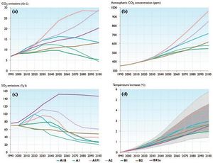
The greatest difference between the SRES scenarios and the earlier IS92 scenarios relates to sulfur emissions and hence sulfate aerosol concentrations. The commonly adopted intermediate IS92 scenario (IS92a) assumed a doubling of anthropogenic sulfur emissions between 1990 and 2050, and little change in emissions thereafter. In contrast, all six illustrative SRES scenarios project lower sulfur emissions in 2100 than at present, although some include an increase over the next few decades. The lower sulfur emissions together with higher GHG emissions in some of the SRES scenarios are the main reason for the upward shift in the IPCC projections of the increase in global mean temperature between 1990 and 2100 from 1.0-3.5°C in the Second Assessment Report[12] to 1.4-5.8°C in the Third Assessment Report[13]. The CO2 emissions and the derived atmospheric CO2 concentrations, the sulfur dioxide (SO2) emissions, and projections of global mean temperature increases for the SRES marker scenarios and for the IS92a scenario are shown in Fig. 4.12.
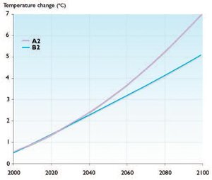
No probabilities are assigned to the various SRES scenarios. During the initial stage of the ACIA process, to stay coordinated with current IPCC efforts, it was agreed that the ACIA projections would be based on the IPCC SRES scenarios[14]. By that time, most of the available (and expected to be shortly available) AOGCM simulations to be relied upon had been forced by two emissions scenarios: A2 and B2[15]. Globally, the model mean transient climate responses to the A2 and B2 emissions scenarios are close to each other for each of the different models through the first half of the 21st century and only diverge significantly after that. Given the schedule for producing this assessment and the limits of resources for data storage, the B2 emissions scenario was chosen as the primary scenario for use in ACIA impact analyses.
In a number of studies[16], a "pattern-scaling" technique is applied to represent a wider range of possible future forcings than are available from AOGCM simulations alone. In particular, Ruosteenoja et al.[17] extrapolated available A2 and B2 AOGCM projections of temperature and precipitation for the SRES B1 and A1FI scenarios over 32 world regions, including the Arctic. The application of this technique is based on the assumption that the spatial pattern of the response is independent of the forcing, while the amplitude of the response at each location is linearly proportional to the global mean change in surface air temperature. The global mean temperature changes for the entire range of SRES scenarios (as shown by shading in Fig. 4.12.d.) were calculated using a simple climate model system calibrated to be consistent with each AOGCM being emulated. Additional assumptions of this approach, first suggested by Santer et al.[18], are that the patterns of the climate response to anthropogenic forcing can be adequately defined from AOGCM simulations and that they are stable through time and across a representative range of possible anthropogenic forcings. Uncertainties due to scaling climate response patterns increase for scenarios that include substantial, regionally differentiated aerosol forcings and in regions where there is an enhanced response, for example, near sea-ice and snow margins[19].
Box 4.4 discusses specific issues related to the use of the ACIA-designated model projections as a basis for local scenarios.
|
Box 4.4. Specific issues related to the use of ACIA-designated AOGCM projections as a basis for local scenarios There are two basic approaches for applying climate change projections in impact studies: deterministic and probabilistic. In the deterministic approach, a single best-guess projection of climate change is used for impact modeling.The simplest way of making a best-guess projection, which is based on the assumption that all models give equally likely results, is to use the arithmetic mean of all available model results (such as the mean of the five ACIA simulations). In the probabilistic approach, in contrast, the projections from different climate models are treated as giving a probability distribution of future climate changes[20]. With this approach, each climate model projection is used separately in an impact analysis. If averaging of different scenarios is performed, it is done in the last phase: the calculated impacts, rather than the climate change projections, are averaged. Because the impacts may depend nonlinearly on changes in climate, the average impact scenario derived by the probabilistic method may differ from the impact scenario obtained by using the average climate change projection. For this reason and because information on uncertainty of the impacts is also important, the probabilistic approach is, in principle, preferable to the deterministic approach. However, it is also more demanding in terms of the computations required. The simplest variants of both deterministic and probabilistic methods assume that all available climate model results are equally likely. In some situations, this simple assumption may be questionable. For example, when models have serious problems in their control climates, it may be best to exclude them from the calculations. Furthermore, for some situations different models may give such widely divergent results that a deterministic averaging may be misleading. Examples of situations in which local scenario construction requires special care include the following.
|
Changes in surface air temperature (4.4.2)
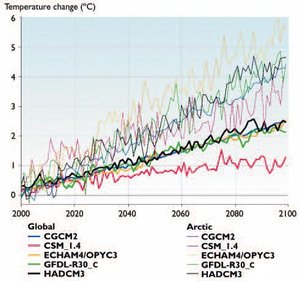
Figure 4.13 displays the evolution of Arctic annual mean temperature during the 21st century projected by the five ACIA-designated model simulations using the B2 emissions scenario. The projections for the 60°-90° N polar region are shown along with the range of global mean temperature changes projected by the same simulations. In the five ACIA-designated model projections, by the late 21st century (2071–2090), the global mean temperature increase (from the 1981–2000 baseline) varies from 1.4°C (CSM_1.4) to 2.1°C (ECHAM4/ OPYC3 and CGCM2), with a five-model average of 1.9°C. In the Arctic, the increase in mean annual temperature projected by the five models is significantly larger, reaching 3.7°C (twice the increase in the global mean) for the area north of 60° N. The projected temperature change varies by about ±25% of the mean of the five models. For the Arctic north of 60° N, the projected area mean temperature increase by 2071– 2090 ranges from 2.8°C (CSM_1.4) to 4.6°C (ECHAM4/OPYC3), with the other models within the 3.7-4.0°C range (Table 4.3). The projected Arctic mean temperature increase exceeds the projected global mean temperature increase in all of the models.
|
Table 4.3. Increases in mean annual surface air temperature in the Arctic (60°-90° N) compared to the 1981-2000 baseline, as projected by the five ACIA-designated models forced with the B2 emissions scenario[21]. | ||||||
|
| ||||||
|
CGM2 |
CSM_1.4 |
ECHAM4/OPYC3 |
GFDL-R30_c |
HadCM3 |
Five-model mean | |
|
2011-2030 |
1.2 |
1.5 |
1.3 |
1.0 |
1.1 |
1.2 |
|
2041-2060 |
2.5 |
2.2 |
3.2 |
2.5 |
2.2 |
2.5 |
|
2071-2090 |
3.7 |
2.8 |
4.6 |
3.8 |
4.0 |
3.7 |
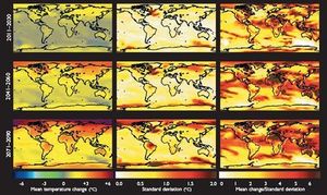
In Fig. 4.14, spatial patterns of projected increases in the annual mean temperature in the Arctic are put in a global perspective for the three 21st-century time slices. On average, the models project a greater temperature increase at high northern latitudes than anywhere else in the world (Fig. 4.14, left column). By 2071– 2090, the five-model average projected increase in the mean annual temperature in the central Arctic is more than 5°C (about three times the global mean). By that time, the mean annual temperature is projected to increase by around 3°C in Scandinavia and East Greenland, about 2°C in Iceland, and up to 5°C in the Canadian Archipelago and Russian Arctic. However, the variation in projected temperature change between the individual models is also generally much larger over the Arctic than for most other regions of the globe (Fig. 4.14, middle column). The standard deviation of the mean temperature change averaged over the five models also varies substantially across the Arctic, but these variations are difficult to interpret because there are only five models in the sample. The relative agreement between the different projections is measured by the ratio between the five-model mean change and the inter-projection standard deviation (Fig. 4.14, right column). Because the large standard deviations compensate for the large average warming, this signal-to-noise ratio in the Arctic is not exceptional. Very high relative agreement (mean exceeding the standard deviation by a factor of six) occurs by 2071–2090 in some (but not all) Arctic regions, but this is also the case in lower latitudes where both the mean and the standard deviation are smaller.
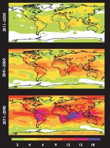
The differences in temperature change between the five ACIA-designated simulations are caused primarily by model differences and by noise associated with internal variability. To investigate the role of the latter factor alone, the five-model mean temperature changes were compared with the variability of 20-year mean temperatures generated in CMIP2 control simulations. The signal-to-noise ratio that was estimated by dividing the average warming by ?2 times the standard deviation of 20-year means is shown in Fig. 4.15. The ratios are generally higher than those in Fig. 4.14, because internal variability does not cause all differences between the ACIA-designated simulations. Importantly, however, the ratio is still relatively low (<2) in some parts of the Arctic in the period 2011–2030. Because a ratio of two defines the lower limit of statistical significance, this suggests that, at least in some parts of the Arctic, the GHG-induced temperature increase may remain difficult to differentiate from natural variability over the next few decades. Indeed, the real signal-to-noise ratio might be even lower than calculated here, because the CMIP2 simulations exclude external sources of natural variability. Later in the 21st century, the signal-to-noise ratio increases, but remains generally lower in the Arctic than at low latitudes, where the internal variability is much smaller. Thus, despite the large average warming suggested by these simulations, the Arctic might not be the area where anthropogenic climate changes are easiest to detect.
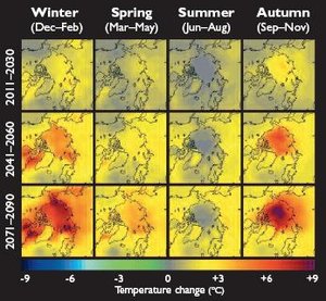
Together, the results in Figs. 4.14 and 4.15 emphasize the importance of improving understanding of how best to interpret the relatively large arctic warming in the light of simulation and projection uncertainties. This issue is discussed further in Section 4.7 (Arctic climate change scenarios for the 21st century projected by the ACIA-designated models). Figure 14.16 displays spatial distributions of seasonal temperature changes in the Arctic for the three 21st-century time slices. The five-model mean projected temperature increase over the central Arctic Ocean is greatest in autumn (up to 9°C by 2071–2090), when the air temperature reacts strongly to reduced sea-ice cover and thickness. Average autumn and winter temperatures are projected to rise by 3 to 5°C over most arctic land areas. By contrast, projected temperature increases over the Arctic Ocean in summer remain below 1°C, because the temperature is held close to the freezing point by the presence of melting ice in both the control and the climate change simulations. The contrast between larger temperature increases in autumn and winter and smaller temperature increases in summer also extends to the surrounding land areas, but is less pronounced there. In summer, projected temperature increases over northern Eurasia and northern North America are larger than over the Arctic Ocean, while in winter the reverse is projected.
The spatial patterns of projected climate change within the Arctic also differ markedly between the individual models, so that, at any single location, the scatter of the model results is larger than it is for change in the arctic area mean temperature. However, all of the models project substantially smaller temperature increases over the northern North Atlantic sector than for other parts of the Arctic. In this area of the sinking branch of the Atlantic thermohaline circulation, the ocean is well mixed to a great depth. Therefore, much of the GHG-induced heating is devoted to warming the deeper ocean, rather than to warming the surface water. The warming is further reduced because the thermohaline circulation weakens in most of the model projections, transporting less warm water from the subtropical regions to the northern North Atlantic. The different degree of projected weakening of the thermohaline circulation in the models presents a special problem for scenario development for the North Atlantic area (see Boxes 4.4 and 4.5).
A comparison between changes in mean annual surface air temperature in the area north of 60° N projected by four of the ACIA-designated models (CGCM2, ECHAM4/OPYC3, GFDL-R30_c, and HadCM3) for the A2 and B2 emissions scenarios is shown in Fig. 4.17. The difference between the two scenarios is not dramatic during the first half of the 21st century, but becomes more systematic and significant during the second half of the century. These differences between the projected A2 and B2 arctic area-averaged temperature increases do not exceed the differences between the highest and lowest projections from the different ACIA-designated AOGCMs.
|
Box 4.5.The Atlantic meridional overturning circulation in the 21st century Evidence from paleoclimate records indicates that the earth underwent large and rapid climate changes during the last glacial and early postglacial periods.The origin of the abrupt changes is being closely studied. A number of studies suggest that the Atlantic meridional overturning circulation (MOC), as part of the global thermohaline circulation, played an active and important role in these rapid climate transitions[22]. Furthermore, modeling studies agree that the Atlantic surface freshwater balance is a key control parameter for the strength and variability of the Atlantic MOC. A common finding from idealized models and AOGCMs is that the strength of the Atlantic MOC decreases if the net flux of freshwater to the high northern latitudes increases[23]. Increased precipitation at high northern latitudes is commonly projected by AOGCM simulations forced with increasing GHG concentrations[24].There is also recent observational evidence of intensification of the hydrological cycle at high northern latitudes[24]. This raises questions about whether the Atlantic MOC will weaken in the 21st century, and what the likelihood is of a full shutdown of the Atlantic MOC. Most AOGCMs forced with prescribed scenarios of the major GHG concentrations and aerosol particle distributions project a weakening of the MOC.The projected changes in the maximum strength of the Atlantic MOC by the end of the 21st century range from about zero to a reduction of 30 to 50%[25]. The projected changes, if any, typically start around 2000 and show a quasi-linear trend thereafter. Irrespective of model differences in the sensitivity of the simulated Atlantic MOC to global climate change, no AOGCM has yet The present generation of AOGCMs used for these simulations does not include freshwater runoff from melting ice sheets and glaciers; therefore, it is possible that the model MOC sensitivity to global climate change is too weak. However, sensitivity experiments with freshwater artificially added to high northern latitudes indicate that fluxes corresponding to several times the present-day freshwater input are required to significantly alter the Atlantic MOC[27], so this shortcoming may not be significant. As a result, the IPCC Third Assessment Report[28] concluded that it is unlikely that the Atlantic MOC will experience a shutdown in the 21st century. It is also likely that the major part of the North Atlantic–Nordic Seas region will experience warming throughout the 21st century, even with a weakened Atlantic MOC. |
Changes in precipitation (4.4.3)
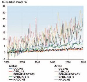
Increases in arctic and global mean annual precipitation over the 21st century projected by the five ACIA-designated models forced with the B2 emissions scenario are displayed in Fig. 4.18. By the end of the 21st century (2071–2090), the projected change in global mean precipitation varies from 1.4% (ECHAM4/ OPYC3) to 4.7% (GFDL-R30_c), with a mean of 2.5%. The Arctic Ocean and terrestrial arctic regions of North America and Eurasia are among the areas with the greatest projected percentage increase in precipitation. The general increase in high-latitude precipitation is a robust and qualitatively well-understood result from climate change experiments. With increasing temperature, the ability of the atmospheric circulation to transport moisture from lower to higher latitudes increases, leading to an increase in precipitation in the polar areas where the local evaporation is relatively small[29].
For the area north of 60° N, all five models simulate an increase in annual precipitation by 2071–2090, which varies from 7.5% (CGCM2) to 18.1% (ECHAM4/ OPYC3), and from 12 to 14% in the other models (Table 4.4). The differences between the models increase rapidly as the spatial domain becomes smaller.
|
Table 4.4. Percentage increases in mean annual precipitation in the Arctic (60°–90° N) compared to the 1981–2000 baseline, as projected by the five ACIA-designated models forced with the B2 emissions scenario[30]. | ||||||
|
Precipitation increase (%) | ||||||
|
CGCM2 |
CSM_1.4 |
ECHAM4/OPYC3 |
GFDL-R30_c |
HadCM3 |
Five-model mean | |
|
2011–2030 |
2.3 |
8.3 |
5.1 |
3.0 |
4.0 |
4.3 |
|
2041–2060 |
4.6 |
8.3 |
12.3 |
7.4 |
7.3 |
7.9 |
|
2071–2090 |
7.5 |
14.0 |
18.1 |
11.9 |
12.9 |
12.3 |
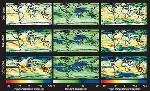
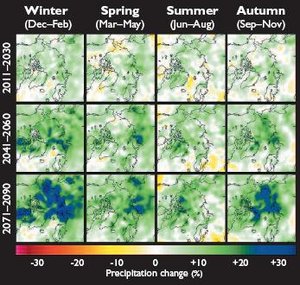
The spatial distribution of the projected mean annual precipitation changes (five-model average) is shown in the left column of Fig. 4.19. By 2071–2090, projected precipitation increases in the Arctic vary from about 5 to 10% in the Atlantic sector to up to 35% locally in the high Arctic. Most of the projected increase in precipitation is due to increasing atmospheric water vapor convergence, which apparently results from the ability of a warmer atmosphere to transport more water vapor from lower to higher latitudes. The increased water vapor convergence is particularly important for precipitation in the high Arctic, where the local evaporation is small (see Section 6.2 (Arctic climate change scenarios for the 21st century projected by the ACIA-designated models)). Although evaporation is projected to increase slightly in most of the Arctic, the change is near zero (or even negative) in the Atlantic sector, where the change in sea surface temperature is small. Unlike surface air temperature, the ratio between the five-model mean precipitation change and the inter-model standard deviation (middle column) is larger in the Arctic than almost anywhere else (right column), with comparable agreement only at high southern latitudes. Nevertheless, the relative agreement between models is worse for precipitation than temperature changes.
Similar to projected temperature increases, the projected increase in precipitation is generally greatest in autumn and winter and smallest in summer (Fig. 4.20), but the summer minimum is less pronounced than that of temperature change.
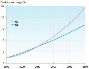
The four-model projected changes in mean annual precipitation for the area north of 60° N (Fig. 4.21) behave similarly to temperature. The difference between the A2 and B2 emissions scenarios is small in the first half of the 21st century. Later in the century, the difference increases and is systematic (i.e., shown in all models), but does not exceed the inter-model scatter.
Changes in other variables (4.4.4)
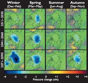
The average projected changes in mean seasonal and annual sea-level pressure are shown in Fig. 4.22.
Throughout the year, there is a slight projected decrease in pressure in the polar region, suggesting a shift toward the positive phase of the AO. However, the changes are small. Even in winter, when the projected decrease in sea-level pressure over the central Arctic is greatest, this amounts to only 4 hPa. The changes projected by individual models are larger, but vary widely, especially in winter. While many impact studies would benefit from projections of wind characteristics and storm tracks in the Arctic, the available analyses in the literature are insufficient to justify any firm conclusions about their possible changes in the 21st century. Changes in cloud cover over the Arctic are small but systematic. By 2071–2090, the five-model average projects an increase in mean annual cloud cover. This is accompanied by a projected decrease (four-model average) in the mean incident short wave radiation. In summer, this flux is projected to decrease across the Arctic by more than 10 W/m2 by 2071–2090 compared to the baseline (1981–2000). The ACIA-designated models agree in their projections of decreases in sea-ice and terrestrial snow extents during the 21st century, as well as general increases both in precipitation minus evaporation over the marine Arctic and in river discharge to the Arctic Ocean from the surrounding terrestrial watersheds. The projected cryospheric and hydrological changes are quantified and discussed in detail in Chapter 6 (Arctic climate change scenarios for the 21st century projected by the ACIA-designated models).
ACIA-designated models in the CMIP2 exercise (4.4.5)
The five ACIA-designated models also participated in the CMIP2 intercomparison[31], together with 14 other models. The model versions used in the CMIP2 simulations are in two cases (CGCM and CSM) slightly different from the ACIA-designated model versions, but this is unlikely to have any substantial influence on the comparison. The CMIP2 intercomparison helps to place the ACIA-designated model results in the broader context of model behavior. The [[climate change]s] in the CMIP2 simulations (Table 4.5) are examined for the 20-year period centered on the year when atmospheric CO2 doubles in the simulations, which takes 70 years in these idealized experiments.
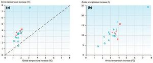
Figure 4.23a shows the global and arctic (60°–90° N) mean temperature changes in the CMIP2 simulations. Models located above the diagonal dashed line project greater temperature increases in the Arctic than globally, while models below the dashed line project the reverse. The global temperature increase varies from 1.1°C (MRI2) to 3.1°C (CCSR2), with a mean of 1.75°C. The mean value for the five ACIA-designated models is very similar but the spread is smaller, 1.4 to 2.0°C. The 19-model average projected increase in mean annual temperature in the Arctic (60°–90° N) is 3.4°C (twice the global mean), and for the five ACIA-designated models the projected arctic temperature increase is 3.6°C. Again, the range of the five ACIA-designated model projections (3.1–4.1°C) is much smaller than the total range (1.5–7.6°C) of all 19 CMIP2 simulations. However, individual outliers contribute substantially to the large range in the CMIP2 results.
|
Table 4.5. The 19 models participating in the CMIP2 intercomparison, with the five ACIA models shown in bold. The first column provides the symbol used in Figure 4.23. | |||
|
Model acronym |
Institution |
Reference | |
|
A |
BMRC |
Bureau of Meteorology Research Center |
|
|
B |
CCCmaa |
Canadian Centre for Climate Modelling and Analysis |
|
|
C |
CCSR1 |
Center for Climate System Research |
|
|
D |
CCSR2 |
Center for Climate System Research |
|
|
E |
CERFACS |
Centre Européen de Reserche et de Formation Avancée en Calcul |
|
|
F |
CSIRO |
Commonwealth Scientific and Industrial Research Organization |
|
|
G |
ECHAM3 |
Max-Planck Institute for Meteorology |
|
|
H |
ECHAM4/OPYC3 |
Max-Planck Institute for Meteorology |
|
|
I |
GFDL-R15 |
Geophysical Fluid Dynamics Laboratory |
|
|
J |
GFDL-R30_c |
Geophysical Fluid Dynamics Laboratory |
|
|
K |
GISS |
Goddard Institute for Space Studies |
|
|
L |
HadCM2 |
Hadley Centre for Climate Prediction and Research |
|
|
M |
HadCM3 |
Hadley Centre for Climate Prediction and Research |
|
|
N |
IAP/LASG |
Institute of Atmospheric Physics, Chinese Academy of Sciences |
|
|
O |
LMD/IPSL |
Laboratoire de Metéorologie Dynamique, Institut Pierre Simon Laplace |
|
|
P |
MRI1 |
Meteorological Research Institute |
|
|
Q |
MRI2 |
Meteorological Research Institute |
|
|
R |
NCAR-CSMa |
National Center for Atmospheric Research |
|
|
S |
NCAR/DOE-PCM |
National Center for Atmospheric Research/ Department of Energy |
|
|
aAn earlier model version than that used by the ACIA participated in the CMIP2 intercomparison. | |||
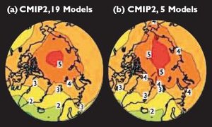
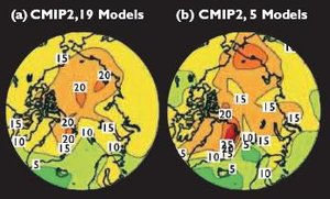
Similar conclusions are valid for the projected change in arctic mean precipitation (Fig. 4.23b). The full range of projected precipitation change in the 19 models (4–24%) is wider than the range in the five ACIA-designated models (8–15%), but the 5-model and the 19-model means are both 11%. The larger set of models shows an expected tendency for the projected precipitation change to be greatest for the models with the greatest projected temperature increase, which is not visible in the results from the five ACIA-designated models alone. The same tendency is seen in a comparison of projected global mean temperature and precipitation change[51]. Figure 4.24 shows the spatial distribution of the projected change in mean annual temperature from the CMIP2 experiments, as averaged over all 19 models and over the five ACIA-designated models. The basic patterns are very similar, with the greatest temperature increases over the central Arctic in both cases. A similar comparison of projected precipitation changes (Fig. 4.25) also indicates broad agreement between the 19-model mean and the 5-model mean. However, some of the spatial details in the 5-model mean, such as the maxima over northeastern Greenland and eastern Siberia, are smoothed out when the change is averaged over all 19 models.
Summary (4.4.6)
Projections of arctic climate change in the 21st century from all of the ACIA-designated AOGCMs are qualitatively consistent and in line with the IPCC conclusions listed at the beginning of Section 4.4 (Arctic climate change scenarios for the 21st century projected by the ACIA-designated models). The across-model scatter of the arctic climate change scenarios is significant, but smaller than the scatter between the climates simulated by the different models for the baseline period. Even the difference between the two single-model projections driven with both the A2 and B2 emissions scenarios is comparable to the range of corresponding changes projected by the five ACIA-designated models forced with the B2 emissions scenario. In summary, the five ACIA-designated AOGCMs appear to be a representative sample of climate models, at least in terms of the average response of arctic temperature and precipitation to the B2 emissions scenario. However, this set of projections does not capture the full range of uncertainty associated with model and emissions scenario differences, at least in the second half of the 21st century.
Chapter 4: Future Climate Change: Modeling and Scenarios for the Arctic
4.1. Introduction (Arctic climate change scenarios for the 21st century projected by the ACIA-designated models)
4.2. Global coupled atmosphere-ocean general circulation models
4.3. Simulation of observed arctic climate with the ACIA designated models
4.4. Arctic climate change scenarios for the 21st century projected by the ACIA-designated models
4.5. Regional modeling of the Arctic
4.6. Statistical downscaling approach and downscaling of AOGCM climate change projections
4.7. Outlook for improving climate change projections for the Arctic
References
Citation
Committee, I. (2012). Arctic climate change scenarios for the 21st century projected by the ACIA-designated models. Retrieved from http://editors.eol.org/eoearth/wiki/Arctic_climate_change_scenarios_for_the_21st_century_projected_by_the_ACIA-designated_models- ↑ Ibid.
- ↑ Ibid.
- ↑ Ibid.
- ↑ Nakicenovic, N. and R. Swart (eds.), 2000. Intergovernmental Panel on Climate Change, Special Report on Emissions Scenarios. Cambridge University Press, 599pp.;-- see also Section 4.4.1
- ↑ e.g., Stocker,T.F., G.K.C. Clarke, H. Le Treut, R.S. Lindzen,V.P. Meleshko, R.K. Mugara,T.N. Palmer, R.T. Pierrehumbert, P.J. Sellers, K.E. Trenberth and J.Willebrand, 2001. Physical climate processes and feedbacks. In: J.T. Houghton,Y. Ding, D.J. Griggs, M. Noguer, P.J. van der Linden, X. Dai, K. Maskell and C.A. Johnson (eds.), pp. 418–470. Climate Change 2001:The Scientific Basis. Contribution of Working Group I to the Third Assessment Report of the Intergovernmental Panel on Climate Change. Cambridge University Press.
- ↑ Mearns, L.O., M. Hulme,T.R. Carter, R. Leemans, M. Lal and P.Whetton, 2001. Climate scenario development. In: J.T. Houghton,Y. Ding, D.J. Griggs, M. Noguer, P.J. van der Linden, X. Dai, K. Maskell and C.A. Johnson (eds.). pp. 739–768. Climate Change 2001:The Scientific Basis. Contribution of Working Group I to the Third Assessment Report of the Intergovernmental Panel on Climate Change. Cambridge University Press.
- ↑ Meehl, G.A., G.J. Boer, C. Covey, M. Latif and R.J. Stouffer, 2000. The Coupled Model Intercomparison Project (CMIP). Bulletin of the American Meteorological Society, 81:313–318.
- ↑ Leggett, J.W., J. Pepper and R.J. Swart, 1992. Emission scenarios for the IPCC: an update. In: J.T. Houghton, B.A. Callander and S.K. Varney (eds.). Climate Change 1992. The Supplementary Report to the IPCC Scientific Assessment, pp. 69–95. Cambridge University Press.
- ↑ Nakicenovic, N. and R. Swart (eds.), 2000. Intergovernmental Panel on Climate Change, Special Report on Emissions Scenarios. Cambridge University Press, 599pp.
- ↑ IPCC, 2001. Climate Change 2001: The Scientific Basis. Contribution of Working Group I to the Third Assessment Report of the Intergovernmental Panel on Climate Change. J.T. Houghton, Y. Ding, D.J. Griggs, M. Noguer, P.J. van der Linden, X. Dai, K. Maskell and C.A. Johnson (eds.). Intergovernmental Panel on Climate Change. Cambridge University Press, 881pp.
- ↑ Ibid.
- ↑ IPCC, 1996. Climate Change 1995: The Science of Climate Change. Contribution of Working Group I to the Second Assessment Report of the Intergovernmental Panel on Climate Change. J.T. Houghton, L.G. Meira Filho, B.A. Callander, N. Harris, A. Kattenberg and K. Maskell (eds.). Intergovernmental Panel on Climate Change. Cambridge University Press, 572pp.
- ↑ IPCC, 2001. Op. cit.
- ↑ Källén, E., V. Kattsov, J. Walsh and E. Weatherhead, 2001. Report from the Arctic Climate Impact Assessment Modeling and Scenarios Workshop. Stockholm, January 29–31 2001. 35pp.
- ↑ Cubasch, U., G.A. Meehl, G.J. Boer, R.J. Stouffer, M. Dix, A. Noda, C.A. Senior, S. Raper and K.S. Yap, 2001. Projections of future climate change. In: J.T. Houghton, Y. Ding, D.J. Griggs, M. Noguer, P.J. van der Linden, X. Dai, K. Maskell and C.A. Johnson (eds.). Climate Change 2001: The Scientific Basis, pp. 526–582.
- ↑ Carter, T.R., M. Hulme, J.F. Crossley, S. Malyshev, M.G. New, M.E. Schlesinger and H. Tuomenvirta, 2000. Climate Change in the 21st Century – Interim Characterizations based on the New IPCC Emissions Scenarios. The Finnish Environment 433, Finnish Environment Institute, Helsinki, 148pp.–Ruosteenoja, K., T.R. Carter, K. Jylhä and H. Tuomenvirta, 2003. Future climate in world regions: an intercomparison of model-based projections for the new IPCC emissions scenarios. The Finnish Environment 644, Finnish Environment Institute.
- ↑ Ruosteenoja, K., T.R. Carter, K. Jylhä and H. Tuomenvirta, 2003. Future climate in world regions: an intercomparison of model-based projections for the new IPCC emissions scenarios. The Finnish Environment 644, Finnish Environment Institute.
- ↑ Santer, B.D., T.M.L. Wigley, M.E. Schlesinger and J.F.B. Mitchell, 1990. Developing climate scenarios from equilibrium GCM results. MPI Rep. 47, Max Planck Institute for Meteorology, Hamburg, 29pp.
- ↑ Carter, T.R., M. Hulme, J.F. Crossley, S. Malyshev, M.G. New, M.E. Schlesinger and H. Tuomenvirta, 2000. Climate Change in the 21st Century – Interim Characterizations based on the New IPCC Emissions Scenarios. The Finnish Environment 433, Finnish Environment Institute, Helsinki, 148pp.
- ↑ (Giorgi, F. and L.O. Mearns, 2003. Probability of regional climate change calculated using the Reliabibility Ensemble Averaging (REA) method. Geophysical Research Letters, 30(12):311–314.;-- Palmer,T.N. and J. Räisänen, 2002. Quantifying the risk of extreme seasonal precipitation events in a changing climate. Nature, 415:512–514.;-- Räisänen, J. and T.N. Palmer, 2001. A probability and decision-model analysis of a multi-model ensemble of climate change simulations. Journal of Climate, 14:3212–3226.
- ↑ Kattsov, V.M., S.V. Vavulin, V.A. Govorkova and T.V. Pavlova, 2003. Scenarios of the Arctic climate change in the 21st century. Russian Meteorology and Hydrology, 10:5–19.
- ↑ e.g., Broecker,W.S., 1997. Thermohaline circulation, the achilles heel of our climate system: will man-made CO2 upset the current balance? Science, 278:1582–1588.-- Ganopolski, A. and S. Rahmstorf, 2001. Rapid changes of glacial climate simulated in a coupled climate model. Nature, 409:153–158.
- ↑ Manabe, S. and R.J. Stouffer, 1997. Coupled ocean-atmosphere model response to freshwater input: comparision to Younger Dryas event. Paleoceanography, 12:321–336.;-- Otterå, O.H., H. Drange, M. Bentsen, N.G. Kvamstø and D. Jiang, 2003:The sensitivity of the present day Atlantic meridional overturning circulation to freshwater forcing. Geophysical Research Letters, 30: 1898, doi:101029/2003GL017578.;-- Rind, D., P. deMenocal, G. Russell, S. Sheth, D. Collins, G. Schmidt and J.Teller, 2001. Effects of glacial meltwater in the GISS coupled atmosphere-ocean model 1. North Atlantic Deep Water response. Journal of Geophysical Research, 16:27335–27353.;-- Schiller, A., U. Mikolajewicz and R.Voss, 1997.The stability of the North Atlantic thermohaline circulation in a coupled oceanatmosphere general circulation model. Climate Dynamics, 13:325–347.;-- Vellinga, M., R.A.Wood and J.M. Gregory, 2002. Processes governing the recovery of a perturbed thermohaline circulation in HadCM3. Journal of Climate, 15:764–780.
- ↑ Curry R., B. Dickson and I.Yashayaev, 2003. A change in the freshwater balance of the Atlantic Ocean over the past four decades. Nature, 426:826–829.;-- Dickson, B., I.Yashayaev, J. Meincke, B.Turrell, S. Dye and J. Holfort, 2002. Rapid freshening of the deep North Atlantic Ocean over the past four decades. Nature, 416:832–837.;-- Peterson, B.J., R.M. Holmes, J.W. McClelland, C.J.Vörösmarty, R.B. Lammers, A.I. Shiklomanov, I.A. Shiklomanov and S. Rahmstorf, 2002. Increasing river discharge to the Arctic Ocean. Science, 298:2171–2173.
- ↑ Cubasch et al., 2001, Op. cit.
- ↑ Ibid.
- ↑ Manabe and Stouffer, 1997, Op. cit.;Otterå et al., 2003, Op. cit.;Schiller et al., 1997, Op. cit.;Vellinga et al., 2002, Op. cit.
- ↑ Cubasch et al., 2001, Op. cit.
- ↑ Manabe, S. and R.T. Wetherald, 1975. The effects of doubling the CO2 concentration on the climate of a general circulation model. Journal of Atmospheric Sciences, 32:3–15.
- ↑ Kattsov, et. al. Op. cit.
- ↑ Meehl, G.A., G.J. Boer, C. Covey, M. Latif and R.J. Stouffer, 2000. The Coupled Model Intercomparison Project (CMIP). Bulletin of the American Meteorological Society, 81:313–318.
- ↑ Power, S.B., R.A. Colman, B.J. McAvaney, R.R. Dahni, A.M. Moore and N.R. Smith, 1993.The BMRC coupled atmosphere/ocean/sea-ice model. Bureau of Meteorology Research Centre, Research Rep. 37. Melbourne, 58pp.
- ↑ Flato, G.M., G.J. Boer, W.G. Lee, N.A. McFarlane, D. Ramsden, M.C. Reader and A.J. Weaver, 2000.The Canadian Centre for Climate Modelling and Analysis global coupled model and its climate. Climate Dynamics, 16:451–467.
- ↑ Emori, S., T. Nozawa, A. Abe-Ouchi, A. Numaguti, M. Kimoto and T. Nakajima, 1999. Coupled ocean-atmosphere model experiments of future climate change with an explicit representation of sulfate aerosol scattering. Journal of the Meteorological Society of Japan, 77:1299–1307.
- ↑ Nozawa, T., S. Emori, T. Takemura, T. Nakajima, A. Numaguti, A. Abe-Ouchi and M. Kimoto, 2000. Coupled ocean-atmosphere model experiments of future climate change based on IPCC SRES scenarios. Preprints, Eleventh Symposium on Global Change Studies, 9–14 January 2000, Long Beach, California, pp. 352–355.
- ↑ Barthelet, P., L.Terray and S.Valcke, 1998. Transient CO2 experiment using the ARPEGE/OPAICE non flux corrected coupled model. Geophysical Research Letters, 25:2277–2280.
- ↑ Hirst, A., S.P. O'Farrell and H.B. Gordon, 2000. Comparison of a coupled ocean-atmosphere model with and without oceanic eddy-induced advection. Part I: Ocean spinup and control integrations. Journal of Climate, 13:139–163.
- ↑ Voss, R., R. Sausen and U. Cubasch, 1998. Periodically synchronously coupled integrations with the atmosphere-ocean general circulation model ECHAM3/LSG. Climate Dynamics, 14:249–266.
- ↑ Roeckner, E., L. Bengtsson, J. Feichter, J. Lelieveld and H. Rodhe, 1999.Transient climate change simulations with a coupled atmosphere-ocean GCM including the tropospheric sulfur cycle. Journal of Climate, 12:3004–3032.
- ↑ Manabe, S., R.J. Stouffer, M.J. Spelman and K. Bryan, 1991. Transient responses of a coupled ocean-atmosphere model to gradual changes of atmospheric CO2. Part I: Annual mean response. Journal of Climate, 4:785–818.
- ↑ Knutson, T.R., T.L. Delworth, K.W. Dixon and R.J. Stouffer, 1999. Model assessment of regional surface temperature trends (1949–1997). Journal of Geophysical Research, 104:30981–30996.
- ↑ Russell, G.L. and D. Rind, 1999. Response to CO2 transient increase in the GISS coupled model: regional coolings in a warmer climate. Journal of Climate, 12:531–539.
- ↑ Johns, T.C., R.E. Carnell, J.F. Crossley, J.M. Gregory, J.F.B. Mitchell, C.A. Senior, S.F.B.Tett and R.A.Wood, 1997.The second Hadley Centre coupled atmosphere-ocean GCM: model description, spinup and validation. Climate Dynamics, 13:103–134.
- ↑ Gordon, C., C. Cooper, C.A. Senior, H. Banks, J.M. Gregory, T.C. Johns, J.F.B. Mitchell and R.A. Wood, 2000. The simulation of SST, sea ice extents and ocean heat transports in a version of the Hadley Centre coupled model without flux adjustments. Climate Dynamics, 16:147–168.
- ↑ Zhang, X., S. Guangyu, L. Hui and Y. Yongqiang, 2000. IAP Global Ocean Atmosphere Land System Model. Science Press, Beijing, 352pp.
- ↑ Braconnot, P., O. Marti and S. Joussaume, 1997. Adjustment and feedbacks in a global coupled ocean-atmosphere model. Climate Dynamics, 13:507–519.
- ↑ Tokioka, T., A. Noda, A. Kitoh, Y. Nikaidou, S. Nakagawa, T. Motoi, S. Yukimoto and K.Takata, 1995. A transient CO2 experiment with the MRI CGCM. Quick Report. Journal of the Meteorological Society of Japan, 73(4):817–826.
- ↑ Yukimoto, S., M. Endoh, Y. Kitamura, A. Kitoh, T. Motoi and A. Noda, 2000. ENSO-like interdecadal variability in the Pacific Ocean as simulated in a coupled GCM. Journal of Geophysical Research, 105(D10):13945–13963
- ↑ Boville, B.A. and P.R. Gent, 1998.The NCAR Climate System Model, Version One. Journal of Climate, 11:1115–1130.
- ↑ Washington, W.M., J.W.Weatherly, G.A. Meehl, A.J. Semtner Jr., T.W. Bettge, A.P. Graig, W.G. Strand Jr., J. Arblaster, V.B. Wayland, R. James and Y. Zhang, 2000. Parallel climate model (PCM) control and transient simulations. Climate Dynamics, 16:755–774.
- ↑ Cubasch, U., G.A. Meehl, G.J. Boer, R.J. Stouffer, M. Dix, A. Noda, C.A. Senior, S. Raper and K.S. Yap, 2001. Projections of future climate change. In: J.T. Houghton, Y. Ding, D.J. Griggs, M. Noguer, P.J. van der Linden, X. Dai, K. Maskell and C.A. Johnson (eds.). Climate Change 2001: The Scientific Basis, pp. 526–582. Contribution of Working Group I to the Third Assessment Report of the Intergovernmental Panel on Climate Change. Cambridge University Press.
- ↑ e.g., Räisänen, J., 2001. CO2-induced climate change in the Arctic area in the CMIP2 experiments. SWECLIM Newsletter, 11:23–28.