Earth observation for wetlands delineation
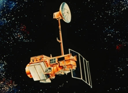
Landsat5 Earth orbiting satellite. Source: National Aeronautics and Space Administration
Earth observation for wetlands delineationinvolves the use of earth orbiting satellites for acquisition of data to map the extent of wetlands. Identification and delineation of wetlands using Earth Observation (EO) technology constitute an important method to perform wetland inventories.
The problem at hand involves the precise delineation of the wetland area, once the location of the wetland is known. Therefore, in this technical note the problem of identification will not be addressed.From an EO perspective the problem of delineating wetlands is rather complex because both the large variation in wetland types, as well as the wide definition of wetlands provided by the Ramsar Convention: i.e., “wetlands are areas of marsh, fen, peatland or other water, whether natural (Natural environment) or artificial, permanent or temporary, with water that is static or flowing, fresh, brackish or saline, including areas of marine water the depth of which at low tide does not exceed six meters. Therefore, a first point in order to define an effective method for delineating wetlands is the precise definition of what should be delineated.
Wetlands are defined in terms of their ecological character. This involves different parameters derived from the hydrological cycle, the vegetation dynamics, the soils and other factors affecting or intervening in the wetland system.
The delineation of the wetland should involve the determination of the geographical area involving all this factors.In this context, EO can only provide a component of the different parameters required to perform this complex task. The final delineation should be carried out incorporating the different layers of information that fully define the ecological character of the site and its dynamics.In this technical note we will address three main approaches with different implications in terms of costs:
- The first is based on the synergic analysis of two main products: a precise Land Cover Land Use (LCLU) map and a Water Cycle Regime (WCR) map together with ancillary information (e.g., DEM, soil types).
- The second approach involves a direct delineation of the areas based on a semi-automatic interpretation of SAR and optical data.
- A third approach is proposed that involves only the mapping of the inundated area. This approach is a simplification of the fist one, where only the inundation information is used as an input. In that case, only the WCR is used to delineate the wetland area. Annex 2 explains the WCR generation.
Contents
Approach 1: Comparing Land Use Land Cover to Water Cycle Regime
The first approach is described in figure 1. As one can see it includes:
|
|
| Figure 1 Annex A provide a description of the LCLU classification process; Annex B provides a description of the WCR generation process |
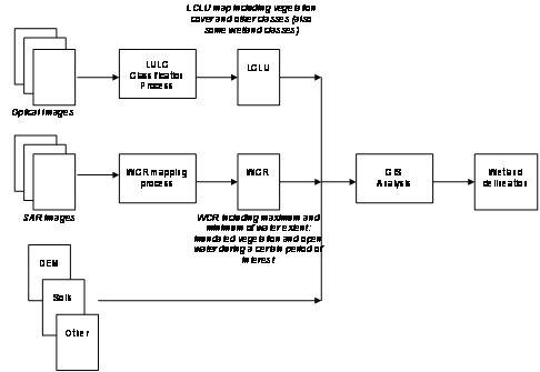
(a) The generation of a Land cover map, which required the availability of suitable ground truth data and an experience operator in remote sensing to derive an accurate final product; The Land Use Land Cover (LULC) map includes a detailed classification of all land parcels within the area of interest at different scales depending on the wetland size (1:5,000, 1:25,000 or 1:50,000).
(b) the production of a water cycle regime map providing an overview of the annual variations of the water table over the wetland site. In particular, this layer, provide at scale 1:50,000 and better, shows the minimum and maximum water extent of the water table, including open water bodies and inundated vegetation, during a hydrological year. This product, when generated over several years, provides wetland managers with a unique monitoring capacity to characterise the water cycle and identify variations that may affect the overall ecosystem.
(c) An synergic analysis of the information together with additional ancillary data;
Approach 2: Interpretation of Optical and SAR Data
In addition to the above method and when the only interested information for delineation is the inundated area and the appearance in the images (therefore without actually taking into account the dynamic ecological characteristics of the site) a detailed delineation can be carried out based on a semi-automatic classification technique.In particular, during the GlobWetland project a delineation approach was developed based on segmentation of both optical and radar images followed by subsequent photo-interpretation of the satellite imagery. The technique used a multi-senor approach based on both optical SPOP-5 data and multi-temporal ASAR imagery. The combination of the two types of images in the interpretation process yielded very good results, in particular, over La Brenne site in central France, where a detailed validation was carried out. A comparison of the GlobWetland map was done versus a very detailed map produced by the French authorities in 1999 using photo interpretation methods of very high resolution aerial imagery. The comparison showed that the total wetland area delineated by the GlobWetland map using satellite imagery was 7159 hectares (ha) versus the 6768 ha derived from aerial photography. This represents an accuracy of 94% in the identification of wetlands. Figure2 shows an example of the product over La Brenne, where blue polygons shows the wetlands identified.
Annex A - Land use and land cover
|
|
| Figure 2. Identification and delineation of Wetlands – La Brenne, France. Source: ESA DUE GlobWetlands project |

The main layer of the GlobWetland information system is the Land Use and Land Cover map, since wetland managers need this type of information to complete or update wetland inventory databases and describe the current status of the wetlands and its surrounding areas.
One of the earliest challenges to generate a standardised data set that could be used worldwide was to define a nomenclature which could be applied across such a broad sampling of wetland types and geographical areas. In this context, a practical approach was applied based on a hierarchical classification of all land cover types (including wetlands) that would enable mapping based on the full range of available EO images. The principal reason to do this was the absence of a single global standard for classifying wetlands as part of whole landscape classification, which was needed to place wetlands in the context of land cover within a catchment context.
The Ramsar classification, widely adopted by Contracting Parties to the Convention, is one solution to the need to subdivide wetlands on the basis of hydro-geomorphology and vegetation, but is not useful for multi-scale EO application. After experiments based on the approach taken by the European countries (which use Corine Land Cover (CLC)), resulting in a hybrid of CLC and Ramsar types at Levels 1, 2 and 3, user feedback strongly indicated that the project should adopt the standard CLC typology using the standard CLC Levels 1, 2 and 3 but with extensions to describe Ramsar wetland types at level 4. This was found to be the most practical solution. In this context, accordingly, the nomenclature adopted was based on CLC, while Ramsar Contracting Parties can relate the legend back to Ramsar wetland types using a simple cross tabulation.
Concerning the classification process, in the last years, many different algorithms and techniques have been tested over wetland areas successfully using both optical and SAR data (Pope et al., 1994; Sader et al., 1995; Augusteijn and Warrender, 1998; Bourgeau-Chavez et al., 2001; Schmidt and Skidmore, 2003; Costa and Telmer, 2006). For the GlobWetland products, an object based approach was selected (Laliberte et. al., 2003; Gitas et. al., 2004; Benz et. al., 2004) because both the capacity of object-oriented methods to extract GIS-ready information (Benz et. al., 2004) and the high accuracies provided by these methods by exploiting the spatial contextual information. Figure 2 summarizes the LULC creation process. The main steps can be summarised as follows.
A segmentation of the original images is carried out to dive the image into “objects” which are groups of pixels who could have similar spectral or shape characteristics (Haralick and Shapiro, 1985; Bénié, 1986; Mansor et al., 2002; Barlow et al., 2003). Following a segmentation process, specific features (e.g., band combinations, texture features characterising the relationships among the different values of neighbouring pixels in the image) were identified to characterise objects and maximize class separability of classes (the distance among classes in the feature space). These features optimize information contained in the objects such as spectral values, shape, texture, hierarchy or thematic attributes (Baatz et al., 2002). Then an automatic supervised classification was applied using different decision rules (e.g., Maximum Likelihood) that allows assigning land cover classes to objects based on the “similarity” of the objects with the ground data information available. The classification process was supported by the commercial software e-Cognition (Benz et. al., 2004).
Some manual editing was done to improve classes such as “Port Areas”, “Airports” and “Industrial Units”, since these land uses are difficult to identify using spectral information alone, therefore it was necessary to exploit the ancillary information available and local knowledge.
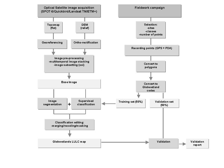 Figure 3. GlobWetland LULC production methodology. Source: ESA DUE GlobWetland Project
It is worth noting that some wetland typologies are difficult to distinguish in the satellite imagery without the support of additional information (e.g. riparian forest vs. mixed deciduous forest, natural grassland vs. pastures). In these cases, manual post-processing of the classification results is required in order to improve the final map. To this end, the resulting classification was exported to a shape-file for further analysis in order to refine the final land cover information manually exploiting the local knowledge provided by wetland managers. Although this manual process is potentially a time consuming exercise, the combination of semi-automated classification together with manual cleaning of problem areas was found to be more efficient than a fully manual interpretation process. This step can in certain cases increase the accuracies of the final results in a 10%.Concerning the selection of the EO data, optical imagery was used as a basis to perform classification. Depending on the wetland size and the required mapping scales, selected images ranged in resolution from less than 1m (Ikonos of Quickbird) to 30m (Landsat TM). In particular, SPOT-5 10m resolution multi-spectral data was well suited to derive LULC maps at the 1:25.000 scale, while Landsat data was used to achieve a 1:50.000 mapping scale. Spatial and spectral resolution in addition to the quality of the supporting data has a direct impact on the quality of the results achieve. After the data were acquired, it was geo-referenced to the national standards of the corresponding countries, ensuring the products were delivered in the end-user’s specified projection. This process is required in order to ensure that end-users could integrate the products with existing raster or vector information. Example of LULC map over Portugal integrated in the GIS system is provided in Figure 4.
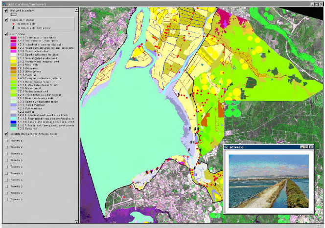 Figure 4: LULC Product over the Tajo Estuary, Portugal. Source: ESA DUE GlobWetland project
Finally, using a GIS, statistics were gathered on the resulting layers providing total areas (in hectares) per classes to create a standard visualization of class composition over a given area. Data were packaged using the ESRI suite of products, into self-extracting archives. The final composite accuracies obtained ranged from 85% to 95%, depending on the type of wetland and the in-situ data available for calibration purposes. In order to summarise some of the findings of the exercise carried out over the 50 GlobWetland sites, the Table below provides an overview of the main challenges faced as well as some strategies applied to solve the problems.
| Challenge | Cause | Solution |
| Limited field work | Lack of resources from end users and project | Work with end users to interpret features on imagery through electronic communications |
| Assignment of classes (how to determine what features to assign to the different classes) | Segmentation provides too many spectral clusters which cannot be logically grouped into classes | Work with the end users, consult supporting material to verify assumptions about class assignment prior to processing data. |
| Separation of natural and agricultural vegetation with very similar spectral properties | Single date optical imagery is limited in its ability to separate these features based on spectral reflectance, in particular SPOT 1-4 and Quickbird which do not have a mid-IR band | Apply some classification rules such as segmentation object’s shape features to look for irregular or regular properties to separate these classes. Also masking areas where different processing is applied can help reduce confusion. |
| Geometric precision and ability to integrate with datasets provided by end users | In some cases, mountainous terrain caused distortions in SAR and Optical imagery; User supplied data was not well documented, projection information was often missing | Establish a base layer at a similar scale as the products which the user can work with, and ensure all derived layers are geometrically registered. |
| Limited ability to capture diversity of land classes in product | Some sites had only a few land cover classes (very homogeneous), lack of detailed site knowledge and supporting data | Work with available material and interact with end users to improve representation of the area in the resulting maps |
| Separating pastures and cultivated land | Single date optical imagery does not give sufficient information to separate these areas – a priori knowledge should be integrated. Alternatively a multi-temporal approach could be used in order to incorporate information of the vegetation spectral response at different stages in the growing cycle. | Work with users to identify some of the parcels, provide them with the option to manually re-assign with the segmentation polygons |
| Determining how to map the transition zone between water and marsh, and marsh and land | The transition zone can be very close spectrally, and is best mapped using multi-temporal imagery | Use SAR to characterise the transition zone to guide process for mapping marshes/water and land classes |
Annex B - Water Cycle Regime (WCR)
Inundated wetland dynamics monitoring using remote sensing has been widely treated in the literature (Al-Khudhairy 2002; Hess et al., 2003; Frazier et. al., 2003; Papa et. al., 2006). This can be done through the estimation of the water levels using altimeter data (Papa et. al., 2006) or by mapping the water table including the open water and the inundated vegetation (Hess et al., 2003). In the context of the GlobWetland project, we focused on the second type of information.Monitoring the water table during a full hydrological year in order to characterise the water cycle of wetlands requires the acquisition of images at different seasons, ranging from the lowest water availability period to the season with the maximum water level and even during flood events. Such image acquisition capacity, especially during flood events or during the rainy season in tropical areas, characterised by abundant cloud coverage, hinders the use of optical sensor and requires the use of SAR data, which is not affected by cloud coverage. Therefore this product relies on the periodical collection of SAR images acquired at critical moments to capture the natural ebb and flow of water in wetlands. The extent of water in wetlands can be easily detected in SAR imagery (Sippel et al., 1994; Melack and Hess, 1998; Prigent et al., 2001) due to the radar response to both open water and inundated vegetation. On the one hand, under low wind conditions, radar reflects on open water as from a mirror, without returning any signal (backscatter) to the sensor. Such lack of backscatter is characterised in the images by a very dark appearance.
On the other hand, due to the double bounce effect created by standing vegetation in water (Henderson et al., 1998), inundated vegetation is easily identifiable under certain conditions of vegetation types, height and density. Through the collection of time series of SAR images, different states can be observed, providing varying backscatter responses from the surfaces imaged. In order to produce the WCR map, a consistent method to analyze the changes was devised. Initially, single pairs of images are considered in isolation of the complete multi-temporal set, which proved to be a challenge since the logical evolution of the water and vegetation classes was difficult to characterize. In order to overcome such limitation, a more robust approach was developed based on a multi-temporal coincident analysis of all SAR images available in a single stack. RADARSAT-1 (C-band, HH polarization, Fine Beam – 10m, 45 degree incidence angle) and ENVISAT ASAR imagery (C-band, HH polarization, Imaging Mode-25m, 30 degree incidence angle) has been used to create these products. Some Alternating Polarization (AP) data was collected from Envisat ASAR (C-band, HV polarization, Imaging mode 30m resolution). The information contained in a single scene of AP data gave an indication of the structure of certain vegetation, particularly in wetland areas due to the differences in backscatter caused by vegetation structure and orientation to the sensor. Further investigation should be carried out to determine optimal acquisition and processing strategies for AP data over wetlands.
- MDA Geospatial Inc., GlobWetland Final Technical Report
- Fitoka E & Keramitsoglou I 2008 (Editors).Inventory, assessment and monitoring of Mediterranean Wetlands: Mapping wetlands using Earth Observation techniques. EKBY & NOA. MedWet publication. (Scientific reviewer Nick J Riddiford).