Deepwater Horizon oil budget calculator

Deepwater Horizon Disaster (main)

Published: January 3, 2011, 12:00 am

Updated: May 4, 2011, 11:20 am

Source: Federal Interagency Solutions Group, Oil Budget Calculator Science and Engineering Team

Topics:

Deepwater Horizon Disaster (main) Oil Spill Response (main) Lessons from the Deepwater Horizon Disaster (main)

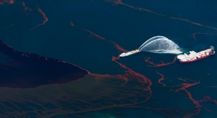
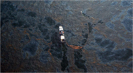
A ship maneuvers and sprays water near a rig in heavy surface oil, as oil continues to leak from the Deepwater Horizon wellhead. Credit: REUTERS/Daniel Beltra/Greenpeace

Editor's Note: This article is excerpted directly from the Federal Interagency Solutions Group, Oil Budget Calculator Science and Engineering Team, "Oil Budget Calculator: Deepwater Horizon," Technical Documentation: a Report to the National Incident Command, November 2010. It has been edited only to conform to the Encyclopedia's style guidelines.

Oil Budget Calculator: Deepwater Horizon, FULLtext (including appendices) - {Download }

Executive Summary

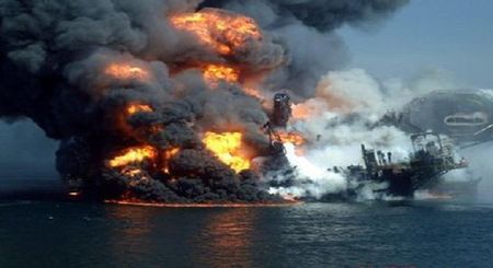The Deepwater Horizon oil platform ablaze on April 21, 2010. Credit: U.S. Coast Guard.

An oil budget (ICS Form 209) is normally prepared as part of the Incident Action Plan for ordinary oil spills. The Deepwater Horizon spill was anything but ordinary, and a special tool had to be developed to construct a workable oil budget useful to the unified command in making its response decisions. This report describes that tool.

The National Incident Command (NIC) assembled several interagency expert scientific teams to estimate the volume of BP Deepwater Horizon oil that has been released from the well and the short-term fate of that oil. The expertise of government scientists serving on these teams was complemented by non-governmental and governmental specialists providing data, offering suggestions, and reviewing the calculations and conclusions.

The Flow Rate Technical Group (FRTG) and the Department of Energy (DOE) developed estimates of the flow rate and of the total volume of oil released. A second interagency team, led by the U. S. Geological Survey (USGS) from the Department of the Interior, and the National Oceanic and Atmospheric Administration (NOAA) and the National Institute of Standards and Technology (NIST) from the Department of Commerce, developed a tool called the Oil Budget Calculator to determine what happened to the oil.

The Oil Budget Calculator was designed to assist the Situation Unit of the Incident Command System (ICS). Therefore, its sole purpose was to inform and advise the response, and it should not be used to assess environmental damage or any other purpose.

The Calculator became operational on June 22, 2010 but continues to undergo modification and refinement, not only best to characterize what happened to the oil in this case, but also to assist in the response to future, similar spill (Oil spill)s. The numbers in this report may change as new information becomes available. The calculator assumed as an input the estimated 4.9 million barrels of oil discharged in total from the well from April 20 until July 14, 2010, provided by FRTG/DOE, and used both direct and indirect measurements and the best scientific estimates available to determine what has happened to the oil.

This report discusses the methods used to estimate the portions of that volume that were recovered directly from the well head, dispersed either chemically or naturally, evaporated or dissolved, burn (Health and safety aspects of in-situ burning of oil)ed or skimmed, and the portion left over (“other” oil) that may still be amenable to response actions. The latest results, by and large, are consistent with early results, produced by an early version of the Calculator and announced in a NOAA (National Oceanic and Atmospheric Administration (NOAA), United States) press release of August 4, 2010: the early estimate of the percentage of “other” (or, “residual”) oil was 26%; the current version of the Calculator estimates it at 23%, and qualifies this estimate with the belief that, with high confidence, the true percentage should be between 11% (best-case scenario) and 30% (worst-case scenario).

The report also describes the methods used to qualify such estimates with uncertainty assessments. Processes such as direct capture and burn (Health and safety aspects of in-situ burning of oil)ing (Health and safety aspects of in-situ burning of oil), that were directly measured onscene, have the smallest uncertainty. Processes such as dispersion (Dispersant use during the BP Deepwater Horizon oil spill) that have to be estimated based upon limited data, theoretical considerations and expert knowledge from past incidents, have the greatest uncertainty. The emphasis was on getting a conservative answer so as not to underestimate cleanup requirements. In terms of response, this translates into using conservative estimates for cleanup efficiency, particularly with regard to skimmer efficiency and dispersant success.

The Calculator does not track the final fate of the spilled oil. Instead it estimates oil that may be amenable to response decisions as opposed to oil that is not (e.g. dissolved or evaporated oil). No attempt was made to estimate the amount of dispersed oil that reached the sediments; nor was degradation rate of any of the oil components evaluated quantitatively. The focus was on estimating the fraction of the spilled oil that might still be amenable to response actions, so that informed decisions could be made.

The Oil Budget Calculator is believed to be sufficiently accurate to meet the needs of the Deepwater Horizon spill response (Stopping the spill: the five-month effort to kill the Macondo well). Thus, while it may have underestimated dispersed oil, it predicted sufficient amounts of subsurface oil as to encourage a large-scale water-sampling program. Suggestions are provided at the end of the report that would allow improved budgets in future large-scale incidents.

Introduction

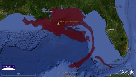Cumulative BP / Deepwater Horizon oil slick footprint (red). Analysis by SkyTruth.

The Oil Budget Calculator grew out of a need to provide status of the spilled oil to the National Incident Command. Excel spreadsheets were first created to record volumes of skimmed oily water, of oil burned, and of dispersant applied. Later, the number of barrels that were directly captured was also recorded. However, there was no accounting for the fate of the remaining oil, and as the model became increasingly complex, the spreadsheets became difficult to interpret. Therefore, the U.S. Geological Survey (USGS), the U. S. Coast Guard, the National Oceanic and Atmospheric Administration (NOAA) and the National Institute of Standards and Technology (NIST) developed the Calculator, using data and supplementary expertise provided by non-government experts. The Calculator became operational, as a response tool, on June 22, 2010. However, it continues to undergo modification and refinement.

This document discusses the technical understanding that was captured in the model implemented in the Calculator — a simplified model that has evolved over time since it was first applied to produce results announced by NOAA (National Oceanic and Atmospheric Administration (NOAA), United States) on August 4, 2010 —, presents an assessment of the oil fate at the time of the well having been capped for good, and gives recommendations for future research. The aforementioned early results (published in a NOAA (National Oceanic and Atmospheric Administration (NOAA), United States) press release) included the estimate of 26% as the percentage of residual or “other” oil. The latest results presented in this report update this estimate to 23%, and assert that, with high confidence, the true percentage should be between 11% (best-case scenario) and 30% (worst-case scenario).

Because this matter has drawn the attention of scholars and other interested parties outside the oil spill science community, additional background material is included. However, in the end, this report is still only the technical documentation of a tool used for response, and it is neither a comprehensive review of the relevant technical literature, nor a research contribution intended for publication in a professional journal. Interested readers seeking more background on oil spill science are referred to Lehr (2001), NRC (2003), or Reed et al. (1999). Appendices describe the statistical approach used to qualify the Calculator’s estimates with uncertainty assessments, the Calculator itself, the raw data used in the Calculator, and supporting findings of laboratory and field studies.

It is important to remember that the Deepwater Horizon incident was an emergency, not an experiment. In spill emergencies, decision makers need immediate information that sometimes requires estimates of unknown quantities without as much data as a scientific study normally would demand. Some of the processes governing the fate of the oil are poorly understood and knowledge about them mostly consists of the personal experience of skilled spill responders. In developing the Calculator, the team handled these poorly understood phenomena by constructing a simplified model that the participating experts could reach a consensus on, or by choosing compromise values (for rate or other constants, for example) if a consensus could not be reached.

The usefulness and accuracy of the Oil Budget Calculator needs to be assessed in light of its purpose, further discussed below. The answers that the Calculator provides to the response team only need to be accurate to the extent that they correctly inform cleanup decisions and do not lead to errors in response actions. Accuracy beyond that level, while desirable from a scientific viewpoint, is superfluous for the purpose for which the tool was designed. Hence, potentially large errors (e.g., in estimates of volumes of dispersed oil) likely would be inconsequential unless they would have led to misdirected response activities: we are not aware of instances of such misdirection in this case.

The reader is cautioned that the numerical values stated in this report are estimates based on the information available at the time that the estimates were produced, and are based on the simplified understanding that the time constraints of the response allowed: therefore, not only are they tentative, but most likely will change as new information becomes available. For this reason, the final mass balance calculation of the Deepwater Horizon Spill lies somewhere in the future, to be produced only after all the appropriate and necessary studies will have been completed.

Purpose and Brief Description of the Oil Budget Calculator

Once spilled into the marine environment and moved from the source, the oil interacts with the environment in a number of processes collectively called weathering (Natural oil degradation processes). Figure 1 shows some short-term processes that acted on this spill (Oil spill)ed oil. These processes change both the composition and properties of the oil, and can result in the amount of oil in the water environment being continually reduced. Other longer-term processes such as biodegradation, photo-oxidation, and sedimentation may have an impact on the environment but are less amenable to response decisions.

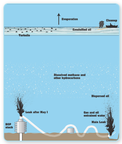Figure 1: Schematic of Deepwater Horizon Oil Spill

The Oil Budget Calculator was designed to assist the Situation Unit of the Incident Command System (ICS). ICS was developed to provide federal, state, and local governments, as well as private and not-for-profit entities, with a consistent framework for the preparation for, response to, and recovery from any incident or event, regardless of the size, nature, duration, location, scope, or complexity. The ICS Form 209 provides the mass balance information that the unified command needs to assess the size of the threat and make informed response decisions. Preparing the mass balance tables for an ICS 209 form is usually a straightforward process. Vessel tanks are sounded, reports from the field estimate oil amount recovered or beached, and standard fate and behavior models, perhaps coupled with trained observer overflights, provide the remaining numbers for the tables. Such was not the case for the recent Deepwater Horizon Spill. Instead, the most sophisticated technology, involving expertise and apparatus never before used on oil spills, was necessary to construct even the most rudimentary mass balance table. The Oil Budget Calculator was a combined effort of several federal agencies, leading academics in the field of spill (Oil spill) science, and practical response experts with years of actual spill (Oil spill) experience. Its results are a product of field measurement, scientific analysis and practical cleanup expertise. The emphasis was on getting a conservative answer. In terms of response, this translates into using conservative estimates for cleanup efficiency, particularly with regard to skimmer efficiency and dispersant success.

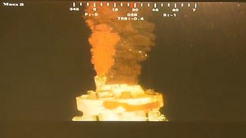A frame from the high resolution video of oil and gas being released from the severed riser pipe on June 3, 2010. Credit: BP

The application of the tool defined its design requirements:

• Calculator must be operable by response personnel, not specialized staff, and use easily accessible input data.
• Calculator must generate output that provides information similar to the standard ICS 209 form along with some estimate of the confidence of the answers generated.
• Calculator must be able to deal with incomplete, uncertain, or missing data and still provide the best estimate available to the unified command.
• The Calculator should be conservative in its answers (i.e., it should err on overestimating oil that is still available to cleanup activities as opposed to oil that is outside of response capabilities).

It is important to understand what the Calculator is not designed to accomplish:

• The Calculator is not a spill research tool, although new research has been a product of its development. Simplifications were made to make it accessible to response personnel.
• The Calculator is not a damage assessment tool and is not applicable to determining environmental impact of the spill (Oil spill)ed oil. Other methods are required for this task.
• The Calculator does not track the final fate of the spill (Oil spill)ed oil. Instead it estimates oil that may be amenable to response decisions as opposed to oil that is not (e.g. dissolved or evaporated oil).

The logical structure of the algorithm that drives the Calculator is straightforward. Mass is conserved as processes act upon the spill (Oil spill)ed oil. The chronological order that is assumed for the unfolding of these processes is based on observations from other spill (Oil spill)s and our understanding of the corresponding science. Oil that comes from the well either is directly captured or not. The portion that is not captured there, in turn either is dispersed naturally or chemically in the jet zone at the leakage points, or rises to the surface. Some of the dispersed oil dissolves into the water column. Some of the oil that floats to the sea surface either dissolves on the way up or quickly evaporates. Oil that remains on the surface can be burn (Health and safety aspects of in-situ burning of oil)ed or skimmed. Some of the surface oil disperses naturally or chemically into the water column. After all these processes, there will be some oil left. A brief description of the governing equations (listed in full in Appendix 1 of the full report) is given below.

(1) Subtract off direct recovery from the total amount escaping from the reservoir. While this oil does not enter the Gulf waters, it was important to record this amount for the Unified Command since logistical assignments depend upon it. If V_R(t) is the oil volume discharged on day t and V_DT(t) is the amount of oil directly recovered, then the effective discharge, V_RE(t), is given by

(2) Determine the lower water column chemical dispersion amount. The amount of oil that is dispersed as a result of the injection of [[dispersant]s] is calculated. To guarantee that mass balance is maintained, this amount cannot exceed the effective discharge. Some of the oil that is dispersed (Dispersant use during the BP Deepwater Horizon oil spill) as small droplets will have a portion of the hydrocarbons dissolve into the surrounding water. Subtracting this gives V_DC(t), the net [[chemically] dispersed oil]:

Here, V_CB(t) is the volume of dispersing chemicals injected into the subsurface jet. The rate constants k₂ and k₇ are defined in Appendix 1 along with the other rate constants. They are treated as random variables whose probability distributions describe our incomplete knowledge about their values, which is a consequence of our uncertainty about the exact attributes of the physical process the equations attempt to model.

(3) Determine natural dispersion from the leaking jet. From oil that is not [[chemically] dispersed], compute the fraction that is [[naturally] dispersed]. Again, subtract oil that dissolves from the droplets.

(4) Calculate the dispersed oil near the bottom. Add the amount that is [[chemically] dispersed] and [[naturally] dispersed] near the bottom. This oil is not available for evaporation, nor is the oil that dissolved near the bottom.

(5) Compute skimmed oil as a fraction of oily water recovered. Not all the liquid recovered by mechanical recovery, V_OW , is oil. The rate constant k₆ specifies that fraction. V_NW(t) = k₆V_OW(t) defines the net skimmed oil. Oil at all stages of weathering is skimmed. The model makes the assumption that the majority of the skimmed oil is "older" oil. Hence, this oil is assumed to have already lost all oil that might evaporate.

(6) Determine oil that evaporates or dissolves. Compute oil that [[evaporate]s] from surface oil during its first day on the surface or dissolves. Add evaporation from the second day on the surface plus oil that dissolves from dispersed oil. Let Z = V_RE(t) - V_DB(t)/(1 - k₇) be the oil that makes it to the surface on day t. The oil that rose to the surface on day t-1 and is still left (neglecting natural surface dispersion and skimming) is W(t - 1) = (1 - k₄)Z(t - 1) - V_BU(t - 1). Since evaporation and dissolution are combined, dissolution from the bottom is added to V_E, the net [[evaporate]d] or dissolved, where

Here V_BU is the volume of oil that is [[burn (Health and safety aspects of in-situ burning of oil)ed] in-situ]. The model uses reported values for daily volumes burn (Health and safety aspects of in-situ burning of oil)ed as one of its inputs. Since the burn (Health and safety aspects of in-situ burning of oil)s involve oil that will have reached the surface at any prior point in time, occasionally the total volume burn (Health and safety aspects of in-situ burning of oil)ed on a particular day may exceed the amount of oil surfacing on that day.

(7) Determine natural surface dispersion. Surface dispersion, V_NS, is a competitive process with emulsification and the potential for dispersion (Natural oil degradation processes) decreases as the oil weathers (Natural oil degradation processes) on the surface. Disperse the surface oil that is available for surface dispersion, after subtracting evaporation and burn (Health and safety aspects of in-situ burning of oil)ing (Health and safety aspects of in-situ burning of oil):

(8) Determine chemically dispersed oil near the surface. Compute volume of [[chemically] dispersed] oil from surfactants sprayed on the surface slicks, V_DS(t). Check that it does not exceed oil volume on the surface, based upon V_S(t - 1), which is the total volume of surface oil remaining from the day before.

Here, V_CS(t) is the volume of [[dispersant]s] used on day t. The remainder is then added to the “Other” oil category. For the purpose of the Calculator, this “Other” oil is treated as if it is all on the surface, when in fact some of it is not.

Appendix 1 lists all the equations used in the current version of the calculator, and explains how the uncertainty assessments for the estimates were produced. The corresponding results are described in Appendix 2, and are summarized in Figures 12 and 13.

Previous Experience - The Ixtoc Spill

The Deepwater Horizon incident is not the first large oil spill in the Gulf of Mexico. In June of 1979, the Ixtoc I exploratory well in the Bay of Campeche blew out, releasing oil for 290 days. It was the largest spill in history, at that time, totaling approximately 3.5 million barrels. The well was in much shallower water (165 ft) than the Deepwater Horizon.

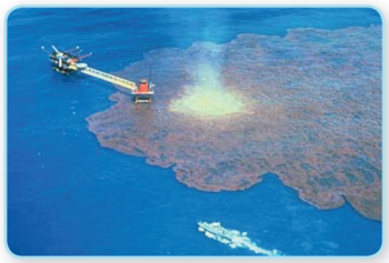Figure 2: Ixtoc I Oil Spill

In many ways, the present Deepwater Horizon spill and response is similar to Ixtoc incident. For example, in both cases the oil released at the well was saturated with gas and formed an emulsion on the surface. In terms of the response, various devices were employed at the Ixtoc and Deepwater Horizon but were unsuccessful at stopping the flow of oil from the well. Again in both situations, eventually a relief well was employed to stem the flow. As for countermeasures, literature states mechanical recovery removed about 4-5% of the oil from the water surface during Ixtoc, which appears similar to the Deepwater Horizon incident. Large-scale [[dispersant] operations] were undertaken on oil on the water surface. In both events there was an impact on the fishing industry from the outright ban or local restrictions on fishing.

As much as the two incidents were similar, there are key differences. It is not the objective of this report to directly compare the two spills. However, as it relates to the subsequent discussion of the Oil Budget Calculator it is important to mention some pertinent detail.

Based on a limited literature review, the obvious difference is the depth of the oil release point where the Ixtoc I release point was approximately 165 ft (51m) below the water surface and the [[Deepwater Horizon] release]point was approximately 5000 ft. (1500m) below the water surface. Second, [[dispersant]s] were used on the surface oil slick at the Ixtoc I but no subsurface application is noted (Jernelov and Linden, 1981). The loss to evaporation to the atmosphere of the [[Ixtoc I] oil] was reported as 50%. It is postulated that the circumstance of the [[Ixtoc I] incident] facilitated a larger mass of the oil reaching the water surface enabling greater overall mass loss to evaporation into the atmosphere in comparison to the conditions at the Deepwater Horizon incident.

There appears to be some differences in the physical and chemical properties of the two oils. Literature (Jernelov and Linden, 1981, Linton and Koons, 1983) noted the [[Ixtoc] oil] was a light type with an API gravity of 32, heavier than the [[Deepwater Horizon] oil]. Detailed chemical analysis of the [[Ixtoc I] well head oil] was not available in the literature reviewed preparing for the Oil Budget Calculator report. The literature did report that the [[Ixtoc I] oil] formed a “chocolate mousse” emulsion on the water surface within kilometers of the wellhead (Overton, 1981). Empirical evidence shows that the Ixtoc I and [[Deepwater Horizon] Macondo] oils differed; this will have some bearing on the mass balance determination of the oil spills.

Finally, literature on the [[Ixtoc I] oil spill] reported that the change in the chemical properties of the spill oil along with the heavy sediment load in the water column caused a good fraction of the oil to settle on the bottom of the [[Gulf] of Mexico]. News reports published in September 2010 indicated that this might also be true for this spill. However, ongoing sampling programs have not confirmed the claim of extensive oil being present on the bottom of the Gulf from Deepwater Horizon.

Jernelov and Linden (1981) constructed the following mass balance table for the [[Ixtoc I] oil spill] which has been included here for the convenience of the readers. It should be noted the table prepared by Jenelov and Linden reports values based on information available at the time. Readers are referred to the literature for further details on the assumptions used and contradictory opinions.

Table 1: Mass Balance for Ixtoc 1

Leak Rate and Subsurface Oil Behavior

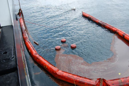
Fishing vessel deploying boom. Credit: Washington Department of Ecology

Oil was initially leaking from two major sources several hundred meters apart. After severing the riser in early June, oil only leaked from the single location at the blowout preventer (BOP). The leak rate varied both in the short-term and in the longer-term. The latter was due mainly to the drop in reservoir pressure. Figure 3 shows the estimated flow rate, based upon studies done by various teams of experts employing a variety of methods. Details on the measurements of the Flow Rate Technical Group (FRTG) Plume Team using image correlation velocimetry are available in the Plume Calculation Team Report (2010). At the time of this document preparation (August and September 2010), the report by the joint effort of the FRTG and Department of Energy (DOE) was still in draft form. The source estimates by FRTG/DOE were considered to be accurate to within ten percent. This uncertainty level is adopted by the Calculator, with three release rates (FRTG/DOE estimate minus ten percent, FRTG/DOE estimate, and FRTG/DOE estimate plus ten percent).

The leak was a combination of gas and oil. In fact, a key parameter in estimating flow was the average ratio of these two. The actual value seemed to vary over the time period of the spill. Increasing gas increased the velocity of the plume but decreased the mass flow. Analysis of available short movies of the riser flow showed the existence of periods when the flow oscillates from pure gas to seemingly pure oil. The DOE/FRTG consensus generally accepted an average value of 44% oil percentage by volume for the exiting flow, based upon measurements of Woods Hole Oceanographic Institute (WHOI, 2010).

The Deepwater Horizon spill was unique not only for its size but also its location at a mile beneath the water surface. In general, when oil and gas are released from a deep-water location, they are expected to break into bubbles or droplets of various sizes. These sizes can vary widely. In field trials off Norway (Chen and Yapa, 2003), they were generally between 1 mm and 10 mm. Leifer (2010) has suggested, however, that the gas bubbles for the Deepwater Horizon spill were smaller than the North Sea (North Sea large marine ecosystem) experiments.

The larger droplets have a relatively stronger buoyancy force to friction force than the smaller droplets (this ratio increases with diameter) and therefore move faster towards the surface than smaller droplets. If the simple form of Stokes’ law is assumed (not valid for larger droplets), droplet rise/fall velocity, ν_rise, is a function of the water viscosity, υ_w, relative density difference, ? ρ, and characteristic droplet size, d. The value of c_stoke varies, depending upon several factors. Figure 4 shows the rise velocity for this oil, according to Yapa et al. (2010).

All the droplets are subject to cross currents that will move them laterally while moving upwards. For this reason the larger droplets and the smaller droplets may not come to the surface at the same location, but quite a distance apart. If there are droplets of very fine scale, it may take weeks or even months for them to come to the surface (Galt, 2010). Galt concluded that even for the large droplets, the rise time was several hours, an answer consistent with Yapa (2010) estimates. Galt also concluded that droplets in the 100 to 200 micron diameter range would take such a long time to surface from a depth of one mile that they were effectively dispersed. This is considerably larger than the common maximum diameter size limit for dispersed oil droplets of around 60-80 microns (Lehr, 2001; NRC 2005). Spaulding et al. (2000) estimated that the rise time for 200 micron droplets with specific gravity of 0.81, less dense than this oil, would have a rise time from this depth on the order of a week.

Figure 3: Estimated flow rate for Deepwater Horizon Spill (DOE/FRTG)

However, the large surface slicks showed that a good percentage of the released oil did make it to the surface. The remote sensing effort of the NASA ER/2 equipped with Airborne Visible InfraRed Imaging Spectrometer (AVIRIS) surveyed about 30% of the core area of the surface spill on May 17, 2010. Extrapolating the examined area to the whole slick, Clark et al (2010) estimated that a minimum of floating oil of between 66,000 and 120,000 bbl. Limitations of the instruments do not allow measurement of very thick oil. The report suggested that if adjustments were made for this limitation, the surface oil could be as much as 500,000 bbl. According to the DOE-FRTG estimates, approximately 1.6 million bbl had been released from the well-head by that time. This suggests that somewhat less than a third of the oil had reached and remained on the surface if the report’s hypothesis is correct. Since sub-surface recovery and [[dispersant] applications] were limited preceding this date, this estimate is not inconsistent with the later estimated values of remaining oil produced by the Oil Budget Calculator.

The plume also contained gas of many bubble sizes. For this incident, a large amount gas bubbles dissolved and may never have made it to the surface. Gas bubbles move faster than oil bubbles if they are the same size. Because of this, gases can separate from the main plume and start going in a slightly different direction (Chen and Yapa, 2004). Gases when released in deep-water, also have the potential to be converted into hydrates. Methane has a level of Hydrate dissociation generally around 550 m of water depth as shown in Figure 5. This is not a fixed value. It depends on parameters like water temperature and gas type (Spaulding et al, 2000). Natural gas can get converted to [[hydrate]s] at a much higher level. Therefore, gases can get converted into [[hydrate]s] as they travel up. Hydrates are still buoyant with specific gravities of around 0.92 to 0.96. As [[hydrate]s] travel towards the water surface they can get reconverted back into gas when they reach the lower pressure in the shallower regions (Leifer, 2010). Where the oil to gas ratio is sufficiently high, rather than an oily bubble, the aggregate is better described as a droplet with internal bubble. He concludes this effect could be very significant. For a primarily gas bubble (i.e., very low oil to gas ratio), in contrast, the effect of surface flow around the bubble pushing surface materials towards the downstream hemisphere could minimize any oil effect. This blowout occurred at far greater pressure than has been studied in the Deep Spill study (Johansen et al. 2000), or the lab (Masutani and Adams (2000), at depths where Hydrate formation is far more rapid (Rehder et al. 2009). The oil budget calculator does not keep track of the gas bubbles, [[hydrate]s] or dissolved gases.

Dissolution

Unlike a typical spill (Oil spill), oil from the Deepwater Horizon spill entered the marine environment 5000 feet below the surface of the Gulf, and started weathering before it reached the airwater surface. Because of the nature of the material flowing from the riser, which was a miscible mixture of oil and natural gas, significant dispersion (Natural oil degradation processes) of the liquid oil occurred near the wellhead. Some of the oil droplets were so small, less than a 100 microns in diameter, that the turbulent diffusivity of the water was enough to overcome the oil’s natural buoyancy, and caused the micro droplets to be dispersed at depth by ocean currents. Larger droplets floated to the surface, however the speed of the transit was determined by the size of the drops. Larger accumulations of droplets of oil rose fairly quickly while smaller droplets rose slowly and were dispersed further from the spill site by currents in the water column.

The important point about this movement of oil from the wellhead is that oil in tiny droplets is exposed to [[weathering] processes] both at depth as well as on its transit to the surface, and once on the surface, weathering continues. Another important point is that much of the oil moved through the marine environment as tiny drops, and these drops were continually exposed to uncontaminated Gulf water in their transit. This means that the dissolution of compounds from the tiny oil droplets was not controlled by equilibrium factors, and this resulted in an almost continuous molecular extraction from the oil droplets by the water column. The results of this continuous extraction are that even sparingly soluble compounds were extracted from the droplets and dissolution was a much more important factor in the weathering of [[Deepwater Horizon spill]ed oil] than it is in more common surface oil spills.

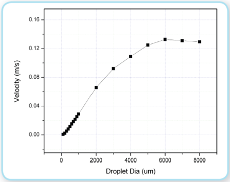Figure 4: Droplet rise velocity (Yapa et al. 2010)

The proverb that oil and water do not mix is usually scientifically accurate when it relates to molecular [[dissolution] of oil] into the surrounding water from a surface spill (Oil spill). For the normal surface type spill (Oil spill), dissolution is less important for estimating the mass balance of the slick (NRC 2003). However, as described above, because of the nature and depth of the release, [[dissolution] of oil] into the water column was a significant weathering factor.

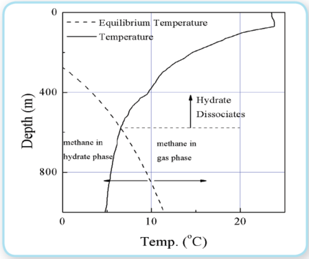Figure 5: A typical ambient temperature and thermodynamic equilibrium curve for Methane (Chen and Yapa 2004)

The dissolution process is a very complex series of interactions between hydrocarbon molecules that are non-polar and surrounding Water molecules that are polar. In general, polar molecules dissolve in polar solvents, seawater in this case, and non-polar molecules dissolve in non-polar solvents, the oil in this case. However, because of their molecular shapes, sizes, and chemical bonds, some non-polar compounds are slightly soluble in polar solvents. Such is the case when considering oil solubility in seawater. As a general rule, small mono-aromatic compounds, such as benzene and the alkyl benzenes, have significant seawater solubility compared to equivalently sized saturated compounds. This solubility extends to larger aromatic compounds, such as naphthalene (Public Health Statement for Naphthalene, 1-Methylnaphthalene, and 2-Methylnaphthalene) and its alkyl homologues, and may also slightly extend to three-ringed aromatic compounds such as the phenanthrenes and the dibenzothiophenes. As a rule of thumb, saturate compounds are the least water soluble of the components of oil, probably because they have no significant interactions with solvent Water molecules and do have significant interactions with similar non-polar compounds in the oil. The conclusions are consistent with experimental results obtained at SINTEF (Melbye at al. 1999) which showed that a component needs to have a water solubility of a minimum 0.3 -1 mg/L in seawater (Figure 6) in order to have any significant potential to dissolve out from an oil droplet when rising to the surface. This means that n-alkanes up to maximum n-C8-9 may have a potential to dissolve but larger alkanes have very limited solubility potentials. However, the mono-aromatic benzene compounds (the BTEX’s), C0- C3 Napthalenes, and the C0-C1-alkylated 3-rings PAH can be stripped out of oil droplets because of their water solubilities. The bottom line is that when tiny droplets of oil transit the water column to the surface, many of the low molecular weight one, two and maybe threeringed aromatic compounds can be dissolved into the water column. This dissolution can affect both the toxicity and physical properties of surface oil from deepwater releases.

Few models or studies exist for oil dissolution at spill (Oil spill)s, mostly in dated work and older generation spill models. Mackay and Shiu (1975) measured the aqueous solubility of fresh and weathered crude oil. Payne et al. (1984) reported that studies of Prudhoe Bay crude found that truly dissolved components were almost exclusively alkyl-substituted lower weight mono-aromatic hydrocarbons with very little n-alkane dissolution. The dissolution rate depends directly upon surface area, which was proportionally larger per volume spilled for this spill incident compared to a normal surface spill (Oil spill) by factors of 100 to 1000. Mackay and Leinonen (1977) concluded that, for droplets less than 100 microns in diameter, dissolution is very rapid for any component that will dissolve at all. Any remaining material in the droplet will consist of relatively insoluble saturate hydrocarbons, i.e. hydrocarbons with a carbon number greater than about 8, and larger multi-ringed aromatic [[PAH]s]. While the droplets that made it to the surface were larger than 100 microns, the extended time that it took for them to reach the surface suggests that dissolution of even marginally soluble compounds occurred.

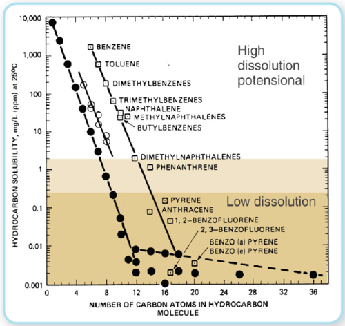Figure 6: Solubility per carbon number for hydrocarbon molecules, (Modified from McAuliffe, 1987 IOSC - proc. Pp 275-288)

It should be pointed out that initial chemical analysis of some samples collected below the Gulf’s surface indicates that significant dissolution did occur. One and two ringed aromatic compounds, and some of the three ringed sulfur heterocyclic aromatic compounds, appear to have been dissolved during transit from the wellhead. These compounds have carbon numbers above 10, and there is some evidence that normal alkanes were also slightly affected by the long transit that occurred as oil drops moved through the water column.

Based upon the chemistry of the oil and the above discussions, it was estimated that any oil exposed to conditions that could lead to dissolution would lose between 5-10% of its volume this way. Since many of these same molecules would evaporate, this process was included in the evaporative losses estimate for any oil that made it to the surface. However, dissolution is subtracted from oil dispersed near the bottom that never reaches the air-water interface. These estimates may change as further studies underway at SINTEF and elsewhere provide additional information. At a minimum, it may be possible to separate dissolved fraction from evaporative fraction. If, on final review, we find that water samples with oil droplets were collected just below the water surface, then by using GC-MS, it is possible to look at the changes in ratios between the more semi-volatile aromatics (e.g. 2-3 rings PAH’s and their alkyl homologues) versus the corresponding n-alkanes with same boiling points (similar vapor pressure, but with far less solubility). In that way, it would be possible to say more specifically how much of the depletion of the components in the range of C10 -C17 is due to dissolution, and how much is due to evaporation. Such information would be useful for impact assessment but, for the purpose of response, would be of limited value. The Oil Budget Calculator groups dissolution and evaporation.

Evaporation

Laboratory and field studies of oil weathering under wide ranging conditions and for a wide range of [[crude oil]s] demonstrate that surface slicks quickly lose volatile components to evaporation. As the more volatile compounds are lost, the rate of evaporation slows. Evaporation is often the most significant loss mechanism from surface slicks during the first week following a spill (Oil spill). Generally, after a week at sea, evaporation is no longer a significant loss mechanism for surface oil. For light crude oils, such as this oil, the great majority of the evaporative loss occurs within a couple days of its exposure to the air.

Empirical methods were used to estimate the evaporation rate during this spill. Samples of weathered oil collected from the sea surface were analyzed using GC/MS. Laboratory weathering of the source oil provided an independent assessment of evaporative behavior. Estimations of evaporation rates were not based on model predictions; rather models were used in analyzing data from field measurements.

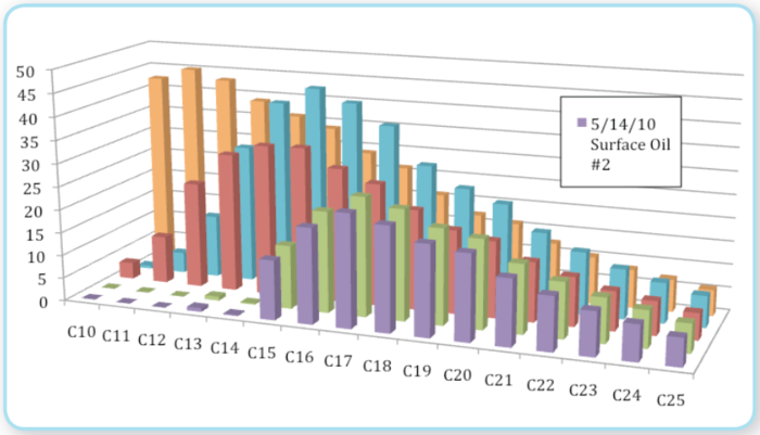Figure 7: Histogram shows the C-10 to C-25 Alkanes of the whole Source Oil (Orange), a floating oil sample immediately adjacent to the source (red), and two floating oil samples at a relatively highly weathered oil further away from the source (green, purple). The highly weathered samples show that virtually all the alkanes below C-15 have been stripped from the original source oil. (Blue bar graph is sample from dispersant efficiency testing).

Evaporation changes not only the volume of a surface oil slick, but changes the chemical composition of the oil as well. Because smaller chemical compounds are preferentially lost during evaporation, it affects the relative abundance of individual chemical compounds within the oil. These changes can be observed by comparing the composition of unweathered oil to that which has weathered on the surface. Other loss processes, such as dissolution, can also change the composition of the oil. While dissolution is usually not a dominant loss mechanism for surface spill (Oil spill)s it might be significant for releases in deep water. Without the appropriate samples, it was not practical to try to resolve the relative importance of dissolution and evaporation, so these two losses are grouped. Oil that never reached the sea surface is not susceptible to evaporative loss, so the measured estimates of fraction [[evaporate]d] only applies to the oil that surfaced.

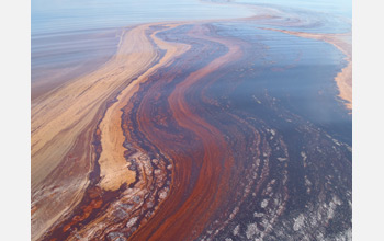Oil slick in the Gulf of Mexico.

Pseudo-component models (Payne et al. 1984; Kirstein et al. 1984) were used to process measured data. These models approximate the oil as an ideal mixture of a relatively small number of components, each component representing a range of individual chemical compounds with similar vapor pressures. Each component is characterized by a mole fraction and a vapor pressure. The rate, per unit area, at which a component [[evaporate]s] from the surface slick is proportional to the wind speed, the mole fraction of that component within the oil (which varies with time), and the vapor pressure of that component (which varies with the temperature of the oil, assumed to be the same as the water temperature). The rate equations for the components are solved simultaneously. The total evaporation rate is set equal to the sum of the rates of the individual components. This method has been adapted for an oil-weathering model, ADIOS2™ , developed by NOAA (Jones 1997), the Type A model developed by ASA (French et al., 1996) and the OWM model developed by SINTEF (Reed, Singsaas et al. 2001).

NOAA (National Oceanic and Atmospheric Administration (NOAA), United States)’s Emergency Response Division (NOAA/ERD) measured the composition of several oils (Figure 7). For the purpose of this discussion on evaporation, in Figure 7 we focus on the oil from the reservoir (Source oil, orange) and the two weathered oils (green and purple) collected from the sea surface on, or around, 16 May. It is not known how long the weathered samples were on the sea surface before being collected. GC/MS analysis was used to measure the relative abundance concentrations of chemical compounds that make up the oil. The weathered oil samples exhibited an expected depletion of the more volatile compounds. The pseudo-component evaporation model used in ADIOS2 (Jones 1997) was initialized with oil-composition data provided by BP in conjunction with oil-composition data measured by NOAA (National Oceanic and Atmospheric Administration (NOAA), United States)/ERD. The ratio of components measured in the more weathered oil samples was compared to those predicted by the model. The extent of evaporative loss was based on the correlation between the measured and modeled ratios. These two weathered oil samples exhibit an average mass loss of 36%. Since the age of these samples is not known, this provides a lower bound on the possible evaporative loss of the surface oil.

SINTEF analyzed three samples of floating oil collected on June 4th and 5th for fraction [[evaporate]d] (Leirvik, Daling et al. 2010). They analyzed the samples by GC/MS and related the fraction [[evaporate]d] to the depletion of alkanes in the C14 to C16 range. They correlated the degree of evaporation with the depletion of these peaks using past results. Their measured data indicated a mass loss to evaporation of 44%, 47%, and 50%. They estimate that the time at sea for these three samples was 1-2 days, 2-3 days, and 4-5 days, respectively.

Laboratory measurements performed by S.L. Ross Environmental Research Ltd. (S.L. Ross Environmental Research Ltd., 2010) on unweathered [[Deepwater Horizon] oil] were consistent with measurements of the above-mentioned surface oil samples. They artificially weathered a 2cm thick slick of [[Deepwater Horizon] oil] in a wind tunnel for 2 weeks. They measured that approximately 35% had evaporated after 2 days, and 45% after 2 weeks. Their measurements exhibit a cumulative evaporation, which is essentially a logarithmic function of time with the majority of the evaporation occurring in the first few days.

Camili et al. (Camili, Reddy et al. 2010) from Woods Hole Oceanographic Institute measured the composition of oil collected from the top 30 m of the water column. They made no attempt to quantify the fractional loss but did attribute the loss of the more volatile compounds to evaporation. Their measurements can be viewed as an additional observation suggesting substantial evaporative loss.

As mentioned above, dissolution also affects oil composition and so losses to dissolution must be considered as contributing to the measured values. Measurements reported here constitute lower bounds to the possible combined losses to evaporation and [[dissolution] of oil] that reached the surface. Loss fractions range from 36% to 50% and are self-consistent. The authors of this report believe that these data provide a close lower bound to the fraction of surface oil lost to the combination of evaporation and dissolution.

The oil budget calculator based the evaporation/dissolution estimates on the compositional change observed in samples of surface oil. It approximates the evaporation/dissolution process as occurring over 2 days; the majority of the loss occurring in the first day. To simplify data entry, requirements to enter variable wind speeds were eliminated. Cumulative evaporation is sensitive to oil composition and temperature but is relatively insensitive to wind speed. The original approximation was 37% lost during the first day (potentially as high as 44% and as low as 33%) with a second day loss of 4% (potentially as high as 6% and as low as 0%). Hence the range of total evaporation of the oil that surfaced was between 37% and 50%. Currently, there is no plan to revise these values.

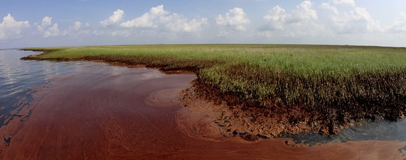Oil from the Deepwater Horizon spill pools against the Louisiana coast along Barataria Bay. Credit: Associated Press

Weathering Estimation by Emulsification

An alternative approach to calculating mass loss has been suggested by Fingas (2010) that uses the fact that the surfacing oil formed emulsions. One important factor to the formation of emulsions is that oils often must weather to a certain percentage before a certain type of emulsion occurs. This is because the asphaltenes and resins must be at a sufficient content to stabilize the oil and also the viscosity must be high enough to retain water droplets long enough for asphaltene/resins stabilization to take place.

Oils from similar oil fields have a tendency to form similar emulsions with similar weathering tendencies. Gulf oils that formed stable emulsions had weathering percentages of 37.7, 26.2, 16.4, 25.5, 22.6, 24, and 35.2%. These average 26.8%. If the [[Deepwater Horizon] oil] shows similar tendencies, the weathering that took place near the release of the Deepwater Horizon was about 16 to 38% with the likelihood that it was near 27%. However, experimental studies by SL Ross Ltd. (see pp. 3 in Appendix 8) and studies at SINTEF showed that an evaporative loss of at least 40-45 wt %, (representing a 200 - 250C+ residue) is needed for this crude oil to start form a significant and stable emulsion. Some additional evaporation would occur as the surface oil moved away from the area, transported by winds and surface currents. Observations of large amounts of emulsified oil indicate that such emulsified oil, at least, had already weathered sufficiently to emulsify.

Natural Dispersion

While the oil released in this spill was buoyant, not all of the oil rose to the surface. Small droplets of oil stayed suspended in the water column just as small dust particles will stay suspended in the atmosphere due to the underlying fluid turbulence. Such droplets will eventually be assimilated through dissolution and biodegradation. They also may become attached to suspended sediment in the water.

Some limited data exists on dispersed oil from the results of RV Brook McCall Survey LISST (Laser In Situ Scattering and Transmissometry) measurements performed by the Bedford Institute of Oceanography (see Appendix 7). It lends support to the hypothesis that much of the oil released was dispersed into the water column. However, since the samples were subsurface, they may be preferentially sampling the droplet distribution with the larger droplets having risen to the surface. Payne’s study reported plumes of oil droplets at depths greater than 2 km. away from the source with larger droplets on the top of the plume and smaller below. This would be consistent with a large amount of dispersion (Natural oil degradation processes) and weak buoyancy. One should be careful about over-interpretation of particle size distribution data that were collected for this specific purpose during the Gulf of Mexico oil spill emergency response operations. Under this emergency response effort, rapid, less than perfect actions had to be taken to support the requirement for immediate action to monitor the fate and transport of the oil.

The NOAA (National Oceanic and Atmospheric Administration (NOAA), United States) oil fate and behavior model, ADIOS2, uses the dispersion formulas developed by Delvigne and Sweeney (1988). These formulas estimate the distribution of droplets sizes based upon the dissipation energy rate e. For most surface spill (Oil spill)s, the turbulent energy comes from breaking waves. Li and Garret (1998) estimate that typical dissipation rates in breaking waves range from 0.1 to 10 m²/sec³ . Others have reported different values. For example, measurements in a wave tank gave values of 0.01 to 0.1 m²/sec³ at the surface (Wickley- Olsen et al., 2007). Field measurements showed lower values varying between about 0.1 and 1 m²/sec³ (Gemmrich and Farmer, 2004, Gemmrich, 2010). Additional information on the value of ε can be found in Kaku et al. (2006).

ADIOS2 suggests that if this spill occurred at the surface under average conditions, only a few percent of the oil would disperse because the oil would emulsify. If emulsification is prevented, natural dispersion could be as much as 30%.

However, it is not breaking waves but the turbulence at the leak that formed these oil droplets. In this case, a new method had to be developed to estimate dispersion (Natural oil degradation processes) rate. ADIOS2, following standard guidelines (NRC 2003), assumes that droplets must be smaller than 70 microns in diameter to be considered permanently dispersed. While appropriate for surface spill (Oil spill)s, it is probably too restrictive for spill (Oil spill)s happening a mile deep. The Calculator uses 100 microns as a cutoff. Based upon the earlier discussion of surfacing time, this was also too restrictive but was consistent with the conservative approach used to calculate oil fate.

Following DS, Q(δ), the entrained droplet mass density for droplets of diameter δ is given by the equation

where C is a constant that depends upon the properties of the oil slick.

For a surface spill (Oil spill), ADIOS2 would expect that the dispersed oil would be

where the bw subscript indicates that this applies to dispersion caused by breaking waves.

If we apply this method to the subsurface leaking pipe (subscript lp) then the same equation would be

and the ratio, R, between the two would be

Thus the estimate of the increase in natural dispersion becomes a problem of estimating ε_lp and ε_bw . Lasheras (2010) has suggested that, to first approximation (Friehe et al. 1972; Gibson, 1963), the maximum theoretical dissipation rate of turbulent kinetic energy can be estimated by

where U_lp is the exit velocity of the flow jet and D_lp is the pipe diameter. He points out that experiments by Martinez –Bazan et al (1999) show that, for distances less than 15 pipe diameters from the orifice, the dissipation rate is much smaller, perhaps as little as 0.02 m²/sec³ . If we take a mid-range value from the Li and Garret suggested bounds for breaking wave dissipation rates compared to the theoretical maximum for ε_lp we get virtually all of the oil naturally dispersing. This obviously does not match observation. If, instead, we use the experimental results of Martinez-Bazan et al., we get approximately 20% subsurface natural dispersion. This more conservative value was used by the Oil Budget Calculator with an assumed maximum of 30% and a minimum of 10%. The minimum value is considered to be the lowest credible estimate consistent with Camilli et al. (2010) and the maximum the largest estimate consistent with the AVIRIS and LISST results.

Lasheras also pointed out that the characteristic size D_char of droplets small enough not to be broken by the turbulent shear forces can be estimated by a simple function of the oil-water surface tension:

This matches the North Sea (North Sea large marine ecosystem) experiments discussed earlier. While the Oil Budget Calculator conservatively assumes that oil that is not dispersed near the bottom would come to the surface, this is not the case. For example, marine snow present in [[Gulf] waters] would scavenge some of the oil droplets on their journey to the surface. The extent of this affect for this spill is uncertain at this time.

Oil droplet size distribution is greatly affected by viscosity and surface tension. Since some of the lighter ends are lost through dissolution on the oil journey to the surface and since the surface oil emulsifies, the viscosity of the surface oil was quite high compared to the oil at the leaking riser. The seas were usually relatively calm, although there were periods of high winds. The original Budget Calculator assumption was that the surface oil would have negligible natural dispersion. This was consistent with the standard to conservatively estimate any reduction in surface oil through either natural or cleanup actions, although certain experts disagreed with this assumption. They pointed out that much of the initial surface oil was not on the surface after storm events. Also, the studies by SINTEF indicate that the weakly emulsified oil is dispersible with enough energy input. Therefore the Calculator was modified to include 5 % natural dispersion of surface oil, based upon ADIOS2 model results. Low value was no dispersion (Natural oil degradation processes) and high value was 10%. As in other dispersion (Natural oil degradation processes) estimations, there was not a uniform consensus by the experts on this revised estimate.

Chemical Dispersion

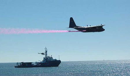
Aerial application of chemical diserpsant to urface oil from the Deepwater Horizon oil platform. Credit: U.S. Coast Guard.

A typical commercial dispersant is a mixture of three types of chemicals; solvents, additives and surfactants. The surfactants are the active ingredient and contain both hydrophobic and hydrophilic groups. This allows them, when coating the oil surface, to reduce its surface tension by as much as a factor of 20 or more, reducing mean droplet size in droplet formation caused by turbulent shearing (Li and Garrett, 1998). Caneveri et al. (1989) measured declines in oil-water interfacial tensions from 18 mN/m without dispersant to 0.1 mN/m with dispersant. More recently Khelifa and So (2009) used a spinning drop instrument to measure declines of oil-brine interfacial tension for three different oils. Declines from 18.3 mN/m without dispersant to 6.5 10-4 mN/m with Corexit 9500 at 1:20 dispersant to oil ratio (DOR) were measured. The same study showed that corresponding droplet size decreases from about 220 mm to 25 mm when the DOR increases from 1:500 to 1:10. (DOR is often expressed with the 1: omitted. Therefore, a DOR of 20 and a DOR of 1:20 refer to the same ratio).

Clayton et al. (1993) noted that successful dispersion of oil in actual dispersant applications only occurs if five requirements are met.

1. The dispersant must reach the oil surface
2. The dispersant must penetrate the oil surface
3. The surfactant must orient at the oil-water interface
4. The surface tension must be reduced
5. Sufficient mixing energy must be applied.

A total of 43,884 barrels of dispersant were used at the DWH incident:

• 18,379 barrels of dispersant were used by sub-sea addition to the discharging oil and gas stream.
  • Initially this was at 12 gallons/minute, later reduced to 7 gallons per minute.
  • The EPA imposed maximum sub-sea use of 15,000 gallons/day (357 bbl/day), equivalent to 10.4 gallons/min
• 25,505 barrels of dispersant were applied to oil on the sea surface (see Figure 8).{| width="200" border="1" cellspacing="1" cellpadding="1" align="center"

| Figure 8: Cumulative dispersant use at the Deepwater Horizon Spill |}

Estimating effectiveness of these dispersant operations was the most difficult challenge in constructing the Budget Calculator, given the present state of oil response technology. As Lewis (2010) points out, the effectiveness of dispersant use at real oil spill incidents cannot be determined by measuring the dispersed-oil-in-water concentration in the water column with sufficient resolution in time or space to produce an accurate mass balance. Nor are there currently commercially available remote sensing techniques capable of measuring oil layer thickness with sufficient accuracy and with sufficient resolution to enable the volume of an oil slick to be determined at any point in time, or how the volume changes with time.

Some surface dispersant applications employed the SMART (2006) protocols. SMART (Special Monitoring of Applied Response Technologies) is a Federal cooperatively designed and regionally approved monitoring program for dispersant operations and in situ burning. However, SMART provides mostly qualitative, not quantitative, estimates of dispersant effectives. SMART teams could at best say that there was some dispersion caused by the dispersant applications.

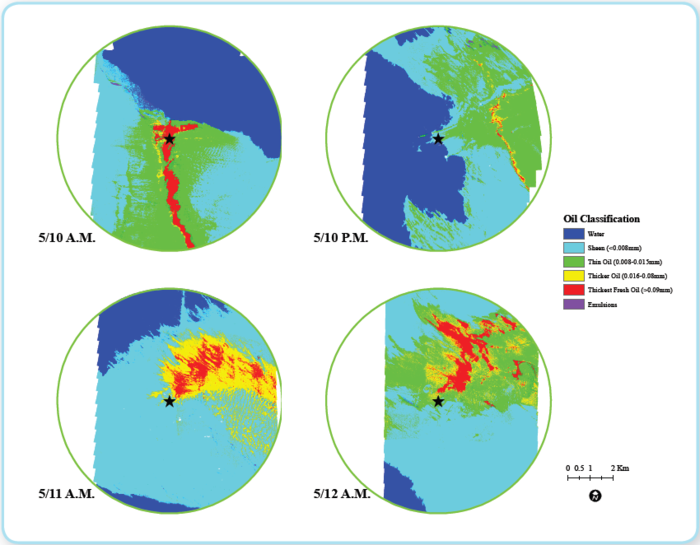Figure 9: Multi-spectral images of the surface oil above leak (Ocean Imaging)

Ocean Imaging, using a multi-spectral scanner to estimate slick coverage at the water surface directly over the spill site, observed the oil appearance both during dispersant operations and no dispersant operations. Figure 11 shows a time period from May 10 through May 12. The individual images represent relative thickness measurements of surface oil at specific times. The larger the red area, the more thick oil is present. Surface conditions were reasonably similar during this time period. Subsurface injection began at 0430 hrs on May 10 and continued with an average injection rate of 8 gallons per minute. If the dispersant was as highly effective as suggested by certain experts, then more than half of the released oil should have been [[chemically] dispersed]. The May 10th A.M. image may be too early to show these results and May 10th P.M. seems to show a drop in surface oil. However, May 11th and May 12th show similar surface expressions although the latter should be displaying more oil. Therefore, these observations provide inconclusive results.

The R/V Brooks McCall field study (Appendix 7) gave some droplet size distribution information but not with sufficient clarity to separate the amount of oil chemically dispersed from the amount of oil naturally dispersed. Analysis was ongoing at the time of preparation of this report and may yet provide useful guidance on this matter.

Given the limited nature of the field data, the best that could be done was to estimate effectiveness using the experience and knowledge of dispersant experts. Unfortunately, reaching consensus among the experts was not possible.

Surface Application

Surface application of dispersant for this spill was extensive. At over 25 thousand bbls, were it a spill by itself, it would be one of the larger spills in U.S. waters. Dispersants were normally applied by aircraft at a dosage of 5 gallons/acre (USGPA) (5000 liter/sq. km). The dosage (DOR) needed to disperse surface emulsions depends highly on the weathering degree (e.g., water content, viscosity) of the emulsion. In Figure 10, controlled laboratory testing shows (and is further discussed in Appendix 6, Figure 4.3) that for the low weathered dark brown (pos. 4) emulsions (i.e., the type of emulsions that the aerial applications was focused on), a very low “absolute” dosage of 1:250 is sufficient in order to disperse the dark emulsion effectively under high mixing energy (breaking waves). This means that an aerial application with typically 5 USGPA is sufficient dosage in order to disperse such dark-brown emulsion with thicknesses around 1 mm as long as the application is efficient and high mixing energy is available. SMART samples similarly show significant dispersed oil in the surrounding water after surface operations in 3 out of 19 samples (see Table 2). When the emulsion become more weathered (i.e. light brown-orange-reddish in color), with a typical water content of >50%, and a significantly higher viscosity, the emulsion was still dispersible under high mixing energy, but a more “traditional” dosage of 1:50 - 1:25 was needed in order to disperse the emulsion effectively using COREXIT 9500. It is probable that some sprayed dispersant missed the oil or was deposited on oil layers that are thinner (such as sheen) or much thicker (emulsified oil) than the nominal 0.1 mm thick oil layer that most dispersant spray systems are designed to treat. Also, the most heavily weathered state of the emulsified oil would impede dispersant success.

Alternative View 1: We believe the Oil Budget Calculator overestimates the effectiveness of chemical dispersants because:

• The WHOI survey and the Ocean Imaging pictures do not support it
• The surface oil was emulsified and there was insufficient mixing in the subsurface injection.

Alternate View 2: We believe that the Oil Budget Calculator underestimates the effectiveness of chemical dispersants because:

• Lab studies show that both the fresh and emulsified oil are dispersible
• There was sufficient energy both subsurface and at the surface to disperse the oil.{| width="200" border="1" cellspacing="1" cellpadding="1" align="center"

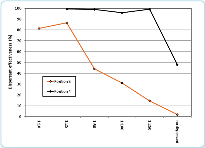| Figure 10: Results from the MNS testing with Corexit 9500 at different dispersant dosages. Position 3 Light brown / reddish emulsion: Viscosity 7200 cP, water content 50%; Position 4: Dark Brown emulsion: Viscosity 1250 cP, water content 33 %. |}

Table 2: USCG Surface Water Dispersant Study Sample Results.

For the reasons stated in the subsurface dispersant application estimation, it was difficult to assess the efficacy of this effort, with a wide variation in the opinions of the experts. As in the case of subsea dispersant operations a compromise value is used in the new version of the Oil Budget Calculator in lieu of a consensus number. The expected DOR is 1:10 with a low value of 1:5 and a high value of 1:20.

Subsurface Application

Measurement of subsurface operation was, at best, highly indirect. The most directly applicable was a published study by Camilli et al. (2010), who reported results from a subsurface hydrocarbon survey using an autonomous underwater vehicles and a ship-cabled sampler. Using BTEX results as an indicator of oil concentration, they concluded that an observed plume of oil at approximately 1100 m. depth represented about 6-7% of the oil leaking from the wellhead. The plume location was consistent with the expected location of subsurface dispersed oil based upon the Clarkson well blowout model (Latimer and Zheng, 2003).

Most of the experts believed that the conditions subsurface were good for dispersant operations. It is likely that all five of the conditions listed by Clayton et al (1993) were generally met. However, the addition of dispersant at 7 to 12 gallons / minute through a narrow diameter wand held by a ROV into the flow of escaping oil and gas would probably not have added dispersant to all of the oil; some oil would have escaped into the water column untreated with any dispersant. Without carrying out some experimentation, it is not possible to say what proportion of the escaping oil would and would not have been treated with dispersant. Also, using the estimated flow rate shown on Figure 3 and the data available on the daily rate of dispersant applications, the dosage of chemical dispersant (DOR) for subsurface application varies from 1:1200 to 1:92; 19% of the time (13 days) the DOR was less than 1:250, 34% of the time (23 days) it was between 1:150 and 1:250 and 43 % of the time (29 days) it was between 1:150 and 1:100. Yet, laboratory studies show that COREXIT 9500 is effective on this type of oil and there was more than sufficient turbulent energy.

The Oil Budget Calculator originally used a very conservative estimate for subsurface dispersant operations. The ITOPF Technical Information Paper for “The use of Chemical Dispersants to Treat Oil Spills” recommends for planning purposes the use of 1 part dispersant for 20 parts oil as the dosage rate. They point out that spraying equipment is often preconfigured to achieve this. Some laboratory studies also support this number (Fingas et al. 1995; Khelifa and So, 2009).

Some experts were concerned that the entrained gas would reduce the effectiveness of the dispersant application by preventing contact between oil and surfactant. They also thought that the time of contact might be insufficient to achieve optimum effect. Their concerns are captured in the choice for minimum effectiveness. However, other experts believe that a 1:20 effectiveness ratio greatly underestimated that actual amount of oil dispersed. They point to successful applications in the North Sea (North Sea large marine ecosystem), producing a larger ratio of dispersed oil to surfactant applied. Ratios as large as DOR 1:100 were suggested. One of the experts was concerned about hydrate interference with dispersant application.

Failing to achieve common agreement of the experts, the new calculator uses a compromise estimate of a DOR of 1:40 with a low estimate of 1:20 and high estimate of 1:90.

Burning

Smoke billows from a controlled burn of spilled oil off the Louisiana coast. Millions of gallons of oil have poured into the Gulf. Credit: GreenEarthAfrica.com

Burning in-situ was extensively used during the Deepwater Horizon Spill. Environmental conditions, location of the incident and the nature of the oil made this possible. Oil was gathered into areas enclosed with special booms and set afire.

For ignition to occur with most oils, the oil film must generally be greater than 2 to 3 mm. Ignition will depend upon the water content of the oil, emulsions of 20 to 25 % or more typically being very difficult to ignite. Since free-floating oil slicks are typically on the order of a tenth of a mm or less, most oil spills need to be contained in special fire-resistant booms. High winds and waves (typically in excess of 1 m short-period, wind waves) may prevent burn (Health and safety aspects of in-situ burning of oil) operations because of the difficulty of preventing entrainment and splash over within the fire boom, and, because of the difficulty of achieving an initial ignition. Most relatively fresh crude oils (even emulsions of 15% to 20% water) may burn with a “thickness reduction” or “regression” rate of approximately 0.05 mm/sec, slightly more than a tenth of an inch per minute (ASTM, 2003). This represents an oil elimination rate of approximately 0.07 gpm/sq.ft. Higher water contents of approximately 25% to 40%, though very difficult to ignite, may burn at rates of approximately 0.05 gpm/sq.ft. During the [[burn (Health and safety aspects of in-situ burning of oil)ing (Health and safety aspects of in-situ burning of oil)] of oil] or emulsions on water, part of the oil is turned into smoke. The actual percentage depends upon the size of the burn and other factors, but usually is in the range of only 5% to 15% of the original volume of oil burned. With typically less than 5 % of the original volume remaining as burn residue, the controlled elimination of spilled oil through combustion is recognized as a highly efficient response option. The burn rates used during the Deepwater Horizon incident range from 0.07 gpm/sq.ft (representing lightly emulsified oils) to 0.05 gpm/sq.ft for burns that may have involved more highly emulsified oils. These oil elimination rates are in line with ASTM standards, and most burn (Health and safety aspects of in-situ burning of oil)s were carried out on emulsions with relatively low water content and along convergence lines where unstable emulsions and wind-herded films had accumulated as dark brown to black oil layers. Daily estimates of the volume of oil burned were recorded as minimum and maximum values reflecting these oil elimination rates. The results were calculated throughout the Deepwater Horizon incident using surface and aerial observations that included the size and duration of each burn. Nearly all burns involved 500-ft-long booms towed in a U-configuration, while attempting to maintain a “gap ratio” (i.e., swath-to-boom-length ratio) of ~ 0.3. A single fire boom could therefore hold 500 to 1000 bbl of oil in its apex, the downstream area only ~1/3 of the way toward the leading ends of the boom. A single burn (Health and safety aspects of in-situ burning of oil) could often eliminate its contents within an hour or less. Field crews concluded that some surface slicks must have been in the range of 2.5 mm to 5 mm to achieve some of the larger burns. This represents a very thick oil emulsion layer.

Figure 11 illustrates the minimum and maximum daily oil elimination rates based upon the burn rates described above. It should be noted that the percentage of burned oil reported by the Calculator applies to all the oil released by the well. If one computes burning share based only upon the volume of available surface oil, the fraction burned is much larger, representing a significant portion of the surface oil. The Oil Budget Calculator uses the range of reported burn values depicted in Figure 11 in its calculations. The uncertainty range for the amount of burned oil is small compared to the other processes discussed in this report.

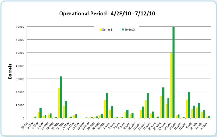Figure 11: In situ burn history for Deepwater Horizon Spill

Mechanical Recovery

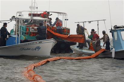Out-of-work fishermen hired by BP laid oil booms yesterday in preparation for the spread of oil in the Gulf of Mexico. Credit: Washington Department of Ecology

Skimmers were the most commonly used mechanical devices use to remove oil from the Gulf water surface. These skimmers varied greatly in size, application, and capacity, as well as in recovery efficiency and water pickup (Schulze, 1993; Schwartze, 1979). In the particular case of the Gulf oil spill the major issue was the amount of water recovered with the skimmed oil. Rather than estimate oil-water ratios, simple measurements of the barge oil would seem the rational way to determine this amount. However, to date, no such measurements are available. Therefore it was necessary to estimate skimmer performance based upon sea conditions, nature of the oil, and past experience.

A skimmer’s performance is affected by a number of factors including the thickness of the oil being recovered, the extent of weathering and emulsification of the oil, the presence of debris, and weather conditions at the time of recovery operations. A skimmer’s overall performance is usually determined by a combination of its recovery rate and the percentage of oil recovered. The maximum amount of oil that a skimmer could recover is called the ‘Nameplate Recovery Rate’ and is typically provided by the manufacturer of a skimmer (Fingas, 2010; Meyer et al, 2009). A similar definition is the ‘Effective Daily Recovery Capacity’, which is the amount that a skimmer could recover in daylight hours under ideal conditions. The recovery rate is the volume of oil recovered under specific conditions. It is measured as volume per unit of time and is usually given as a range. If a skimmer takes in a lot of water, it is detrimental to the overall efficiency of an oil spill recovery operation.

Skimmer performance is chiefly the product of three parameters. The Oil Recovery Rate (ORR) is the quantitative rate in volume per unit time, usually m³/hour and is corrected for water recovery. The throughput efficiency (TE) is applicable only to advancing skimmers. The throughput efficiency is the percentage of oil presented to a skimmer versus that recovered, in percent. The recovery efficiency (RE) is the percent of oil recovered out of the total oil and water recovered. For the Gulf recovery effort, the RE is the most important factor. We know the total liquids recovered, but we do not know exactly how much oil was in this liquid and therefore must estimate the actual oil recovered. Past studies show that the average RE of the skimmers in wave conditions is 33%.

The measured water content of skimmed emulsions varied. An estimate of the actual recovered oil would be a product of the average RE times the oil content of the emulsion. The Calculator assumes that 20% of the skimmed liquid was oil, with a range between 10% and 40%. These are conservative estimates in line with the philosophy behind the Calculator. They are also considered temporary numbers, pending any measurement results.

Other Oil

Oil is collected in skimming boom attached to the USCG Cutter Cypress May 31, 2010. The cutter has been diverted from its routine duties to help with the response to the oil spill. Credit: U.S. Coast Guard

The Oil Budget Calculator does not quantify the amount of oil volume that becomes tar balls, forms surface slicks, sinks due too sedimentation, remains in the surf zone or impacts the shore and is subsequently cleaned up. These are instead grouped together as ‘other oil’.

The amount of oil listed as ‘other’ is quite large. Obviously, there are no longer large surface slicks in the [[Gulf] of Mexico]. So where is this oil? Some obviously did impact the coastline, particularly the Louisiana coastline. Cleanup operations recorded the volume of oil debris that was recovered during shoreline cleanup. However, no estimates were made of the percentage of oil in this debris so it is not possible to give a reliable estimate of this amount. Based upon past spills, the oil content of collected debris mass is only a few percent. Some of the oil may have aggregated with sediment in the water column and settled to the sea bottom. The Oil Budget Calculator does not estimate sedimentation.

Much of this oil probably formed tarballs or millimeter scale oil droplets since the conditions of this spill were conducive to such tarball/droplet formation (turbulent subsurface release, large use of dispersant on weak emulsions, etc). The larger tarballs are very persistent in the marine environment and can travel hundreds of miles, sometimes re-concentrating in convergence zones far from the original spill site. Some limited efforts were made to collect and quantify the larger tar ball mass density in the nearshore areas but the available data was insufficient to make a global estimate. The smaller oil droplets behave in some respects almost as dispersed oil and are similarly subject to biodegradation, dissolution, and sedimentation.

Longer Term Processes

While not tracked by the Oil Budget Calculator, there are other processes that work to break down the [[spill]ed oil (Deepwater Horizon oil spill )]. Two important ones for the [[Gulf] of Mexico] are photo-oxidation and biodegradation.

The combination of hydrocarbons with oxygen is called oxidation. The newly formed oxidized compounds may affect the oil slick by increasing dissolution, dispersion or emulsification. While trace metals in the oil may influence the oxidation process, ultraviolet light significantly increases oxidation. Virtually all of the molecules that evaporate from the slick undergo photochemical oxidation in hours or days. Also, beached oil will show the effects of exposure to sunlight. Even floating oil can show chemical changes due to this process. Overton (1981) exposed IXTOC I crude oil to sunlight and discovered the formation of tarry flakes, showing the involvement of photolysis. Observers at the Mega Borg spill in the Gulf of Mexico noticed the formation of crusts on floating tarmats and tar balls, with the hypothesis that this was due to photo-oxidation.

Hydrocarbons, including those found in oil slicks, are a food source for many microorganisms. The rate of such biodegradation depends upon the availability of nitrogen and phosphorus-containing nutrients in the water, as well as the surface exposure of the oil to the organisms. Swannel and Daniel (1999) suggest that dispersant use on a slick may speed up biodegradation by promoting the growth of indigenous, hydrocarbon-degrading bacteria as well as increasing the surface area of the oil available for microbial colonization.

Bacteria capable of degrading various groups of petroleum hydrocarbons have been found in all oceans and in deep as well as shallow water. Research on biodegradation has occurred with many types of oils and fuels, at temperatures ranging from -1C (polar) to over 30 C (hot, tropical), and at natural oil seeps. Tools for documenting biodegradation rates include microbial taxonomy and abundance, nutrient uptake, oxygen utilization and mass loss.

The [[Deepwater Horizon] blowout] resulted in petroleum hydrocarbon contamination on sand beaches and marshes, at the sea surface, in the warm (30-35C) upper water column adjacent to dispersant operations, and in cold (4.5 to 5C) water at 1100 to 1300 m deep. Available results to date have been reported from surveys conducted in May and June, 2010, and focused on indicators of biodegradation in the contaminated deepwater layers (Camilli et al., 2010 and Hazen et al, 2010).

Camilli et al (2010) reported presence of sub-surface volatile hydrocarbons and also only slight reductions of oxygen at depth and suggested biodegradation rates were low potentially resulting in many months of hydrocarbon persistence. Hazen et al (2010) reported that the dispersed hydrocarbons in deep water originating from the [[Deepwater Horizon] blowout] source stimulated deep-sea indigenous γ-proteobacteria that are closely related to known petroleum-degraders. Hydrocarbon-degrading genes coincided with the concentration of various oil contaminants, namely alkanes. Changes in hydrocarbon composition with distance from the source and incubation experiments with environmental isolates demonstrated faster than expected hydrocarbon biodegradation rates at 5°C. The half-life degradation rates ranged from about 2 to 6 days, depending on the alkane. Based on these results, Hazen et al (2010) concluded that the potential exists for intrinsic bioremediation of the petroleum hydrocarbons in the deep-water column without substantial oxygen drawdown.

Other studies unrelated to this incident have reported a wide range of hydrocarbon degradation rates depending on all the variables indicated above. The Hazen et al (2010) rates are not inconsistent with those published by Venosa and Holder (2007) for cold water using dispersed Alaska North slope crude oil.

Past biodegradation research has focused on marine waters of moderate to warm temperatures, including oil-contaminated sediment interstitial waters of beaches and marshes as well as dispersed/dissolved hydrocarbons. Going back into history, Walker and Colwell (1977) measured the loss of mass South Louisiana crude oil during replicated in situ incubation field experiments in a North Carolina estuary at 30C. The mean mass of 365 mg of oil was reduced to 235 mg in one week (35% reduction), 178.5 mg in 2 weeks 51.1 percent reduction) , 11.2 mg in 3 weeks (97.0 per cent reduction and and 8.8 mg in 4 weeks (97.6 per cent), yielding a half life of about 2 weeks (14 days). Bacteria counts reached maximum in 3 weeks then stared to decline. Presumably, the initial loss of mass was due to evaporation of more volatile components whereas the later stages were the result of biodegradation. These simple rate results fall somewhere between the predictions of Camilli et al (2010) and Hazen et al (2010).

Since the 1970’s, there has been a considerable amount of field, mesocosm, and laboratory work done. The rates resulting from these studies also range widely depending on oil types, oil weathering, dispersion effectiveness, dispersant composition, nutrient loadings, and especially which target petroleum compounds or groups of compounds each research team analyzed. The National Research Council (NRC, 2005) reviewed much of the work done on biodegradation of dispersed oil concluding that most of the work has not been consistently standardized sufficient to confidently extrapolate from the laboratory to the field. Further, there is a paucity of work on degradation of higher molecular weight polycyclic aromatic hydrocarbons, the most toxic compounds. Field studies in contaminated marshes and beach sediments, have demonstrated a wide range of biodegradation rates; oil biodegraded almost completely within a few weeks at some locations while it persisted for tens of years at other locations (Reddy et al., 2002; Short et al, 2004). Boufadel et al., (2010) noted low oxygen and nutrient concentration that might have prevented effective biodegradation of the Exxon Valdez oil spill. The study of Li and Boufadel (2010) highlighted that understanding beach hydraulics is a critical step in predicting the fate of oil within beaches. Therefore, we would expect this oil to undergo biodegradation at different rates in different compartments of the [[Gulf] ecosystem].

Assessment and Future Plans

While pure scientific research can be done on oil spills, most oil spill science is applied science. Tools such as the Oil Budget Calculator are only useful if they provide information that will assist response decisions. Conversely, they need only be as accurate as the precision needed for these decisions. Improved accuracy beyond those levels may be important in the academic sense but not in the response area. Figures 12 and 13, below, show the output from the model, given the revisions described in this document. They vary somewhat from earlier calculations but probably not significantly according to the above criteria.

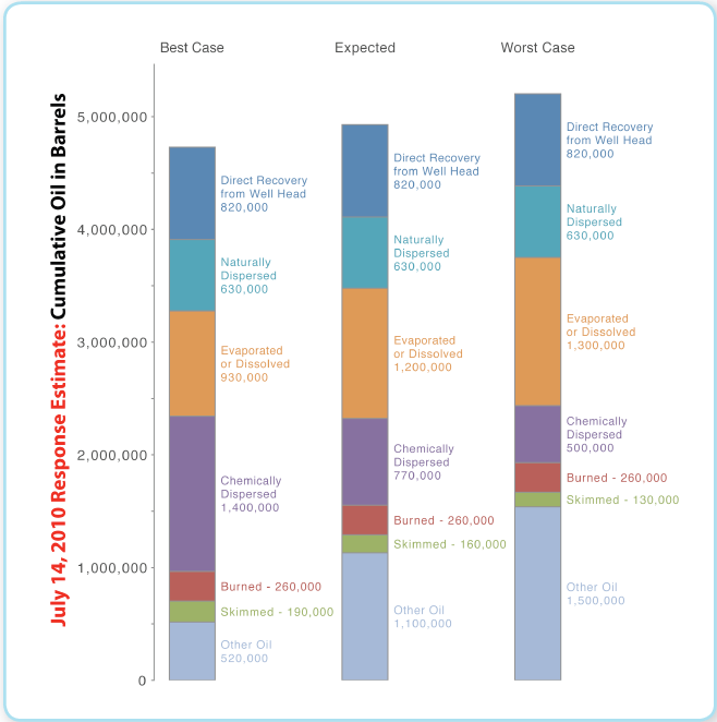
The estimates of the Calculator were admittedly rough for the reasons discussed in this report. However, the estimates were probably sufficient to meet the needs of the Response. Ultimately, of course, that judgment will be made by the NIC. The experience in developing the Calculator points to areas of needed future research and planning:

1. Protocols for surface and subsurface sampling: While oil samples were collected for impact assessment, few samples were properly collected and categorized for response. For example, samples often came from skimming barges, where oil in different states of degradation was blended together. Future response plans should specify methods for gathering proper representative samples.
2. Dispersed oil droplet size: A major improvement in estimating dispersant efficiency would be possible if practical operational tools and methods existed to characterize droplet size distribution of subsurface oil.
3. Basic Models for Longer-term processes: While longer-term processes such as biodegradation often happen outside the time frames of the response, understanding and being able to predict such longer-term changes may be useful in making response decisions.
4. Estimation of collected shoreline oil: For a complete mass balance, procedures should be implemented that estimate the fraction that is oil or oiled debris gathered from shoreline cleanup.
5. Expanded modeling capabilities: Many of the team members that assisted with the Oil Budget Calculator are also part of a working group of spill experts developing the specifications for the next generation of oil spill model. These specifications need to be translated into real code.
6. Revised interface: A better interface is necessary to more properly display the intrinsic uncertainty in the Calculator.{| width="200" border="1" cellspacing="1" cellpadding="1" align="center"

| Figure 13: Response estimates expressed as percentages of the cumulative volume of oil discharged through July 14, 2010, in the best, expected, and worst cases. These estimates served solely as a guide for the national response to the Deepwater Horizon MC252 Gulf Incident. |}

References

Works Cited

• ASTM (2003) F 1788 – 97, Reapproved 2003, Standard Guide for In-Situ Burning of Oil Spills on Water: Environmental and Operational Considerations, 6 pp.
• Boufadel, M. C.; Sharifi, Y.; Van Aken,B.; Wrenn, B.A. and Lee, K. (2010) . “Nutrient and oxygen concentrations within the sediments of an Alaskan beach polluted with the Exxon Valdez oil spill”. Environmental Science and Technology, in press.
• Camilli, R.; Reddy, C.M.; et al. (2010). “Tracking Hydrocarbon Plume Transport and Biodegradation at Deepwater Horizon”. Sciencexpress, 19 Aug. 2010. 10.1126/ science.1195223.
• Caneveri, G.P.; Bock, J; Robbins, M. (1989). “Improved Dispersant Based on Microemulsion Technology”. In: Proc. 1989 International Oil Spill Conf., American Petroleum Institute, Washington, DC. pp. 317-320.
• Chen, F.H.; Yapa, P.D. (2003). “A Model for Simulating Deepwater Oil and Gas Blowouts - Part II : Comparison of Numerical Simulations with “Deepspill” Field Experiments”. Journal of Hydraulic Research, IAHR, August, 41(4), 353-365.
• Chen, F.H. and Yapa, P.D. (2004). “Modeling Gas Separation from a Bent Deepwater Oil and Gas Jet/Plume”. Journal of Marine Systems, Elsevier, the Netherlands, Vol 45 (3-4), 189-203.
• Clark, R.N.; Swayze, G.A.; Leifer, I.; et al. (2010). “A method for quantitative mapping of thick oil spills using imaging spectroscopy”. U.S. Geological Survey Open-File Report 2010–1167, p. 51.
• Clayton, J.; Payne, J.; Farlow, J; Sarwar, C. (1993). Oil Spill Dispersants, Mechanisms of Action and Laboratory Tests. CRC Press, Boca Raton, Fl., pp 113.
• Delvigne, G. A. L.; Sweeney, C.E. (1988). “Natural Dispersion of Oil”. Oil and Chemical Pollution Vol 4, Issue 4, pp 281-310.
• Fingas, M.F., (2010). “Weather Effects on Oil Spill Countermeasures”. Chapter 13 in Oil Spill Science and Technology, p. 339-426.
• Fingas, M.F., D. Kyle and E. Tennyson, Dispersant Effectiveness: Studies into the causes of Effectiveness Variations, in The Use of Chemicals in Oil Spill Response, ASTM STP 1252, 1995, p.92-134.
• French, D.; Reed, M.; Jayko, K.; et al. (1996). The CERCLA type A natural resource damage assessment model for coastal and marine environments (NRDAM/CME), Technical Documentation, Vol. I - V. Final Report, submitted to the Office of Environmental Policy and Compliance, U.S. Dept. of the Interior, Washington, DC, April, 1996; Available from National Technical Information Service, 5285 Port Royal Road, Springfield, VA 22161, PB96-501788.
• Friehe, C. A.; Van Atta, C. W.; Gibson, C. H. (1972). “Jet turbulence: Dissipation rate measurements and correlations”. In Turbulent Shear Flows, AGARD Conference Proceedings, vol. 93, p. 18-1.
• Galt, J. (2010) personal communication to B. Lehr Gemmrich, J., (2010). “Strong Turbulence in the Wave Crest Region”. Journal of Physical Oceanography, Vol. 40, pp. 583-595.
• Gemmrich, J.; Farmer, D.M., (2004). “Near-Surface Turbulence in the Presence of Breaking Waves”. Journal of Physical Oceanography, Vol. 34, pp. 1067-1086.
• Gibson, M. M. (1963). “Spectra of turbulence in a round jet”. Journal of Fluid Mechanics, Vol 15, Issue 2, pp. 161-173.
• Hazen, T.C.; Dubinsky, E.A.; DeSantis, T.Z.; et al. (2010). “Deep-sea Oil Plume Enriches Indigenous Oil-Degrading Bacteria”. Sciencexpress, 24 Aug., 2010, 10.1126/ science.1195223.
• Jernelov, A.; Linden, O. (1981). Ixtoc I: A Case Study of the World’s Largest Oil Spill. Ambio, Vol 10, No. 6, pp. 299-306.
• Johansen, O., et al. (2001), Deep Spill JIP Experimental Discharges of Gas and Oil at Helland Hansen, Parts I, II, and III – Technical Report, SINTEF Applied Chemistry, Norway.
• Jones, R. K. (1997). “A simplified pseudo-component oil evaporation model”. In Proceedings of the 20th Arctic and Marine Oil Spill Program (AMOP) Technical Seminar, Canada, Environment Canada. Pp.43-61.
• Kaku, V. J.; Boufadel, M.C.; Venosa, A.D. (2006). “Evaluation of mixing energy in laboratory flasks used for dispersant effectiveness testing”. Journal of Environmental Engineeering, ASCE 132(1): 93-101, 2006.
• Khelifa A.; So, L.L.C., (2009). “Effects of Chemical Dispersants on Oil Brine Interfacial Tension and Droplet Formation”. In Proceedings of the Thirty-second Arctic and Marine Oil Spill Program (AMOP) Technical Seminar, Environment Canada, Ottawa, Ontario, Vol. 1, pp. 383-396.
• Lasheras J. (2010) personal communication to B. Lehr Latimer, J.S.; Zheng, J. (2003). The sources, transport and fate of PAHs in the marine environment. In: Douben P.E.T. (Ed.). PAHs: an ecotoxicological perspective. John Wiley & sons Ltd., New York, USA. pp.10-22.
• Lehr, W (2001). “Review of the modeling procedures for oil spill weathering behavior, in Oil Spill Modelling and Processes”. C.A. Brebbia (ed), WIT, Press, Southhampton, U.K.
• Leifer, I., (2010). “Characteristics and scaling of bubble plumes from marine hydrocarbon seepage in the Coal Oil Point seep field”. J Geophys Res, In Press, doi:10.1029/2009JC005844.
• Leirvik, F.; Daling, P.; et al. (2010). “Assessment of dispersibility of DWH oil at different stages of weathering”. SINTEF. Marine Environmental Technology.
• Lewis, A. (2010) Estimated Effectiveness of Dispersant Use at the Deepwater Horizon Incident. Unpublished report, 31pp.
• Li. M.; Garret, C. (1998). “The relationship between oil droplet size and upper ocean turbulence”. Marine Pollution Bulletin, Vol. 36, pp. 961-970.
• Li, H.; Boufadel, M.C. (2010). “Long-term persistence of oil from the Exxon Valdez spill in two-layer beaches”. NATURE geosciences, Vol 3, pp. 96-99.
• Linton & Koons (1983). Oil Dispersant Field Evaluation IXTOC I Blowout, Bay of Campeche, Mexico. Oil & Petrochemical Pollution, Vol.1, No. 3. Graham & Trotman Ltd. Vol 1. pp 183-188.
• MacKay, D.; Leinonen, P. (1975). “Mathematical model of the behavior of oil spills on water with natural and chemical dispersion”. Report No EPS-3-EC-77-19, Environment Protection Service: Ottawa, Canada 84 pp.
• Mackay, D.; P. J. Leinonen. 1977. “Mathematical Model of the Behavior of Oil Spills On Water with Natural and Chemical Dispersion”. Prepared for Fisheries and Environment Canada, Economic and Technical Review Report EPS-3-EC-77-19.
• Mackay D.; Shiu W. Y. (1975). “Determination of the solubility of hydrocarbons in aqueous sodium chloride solutions”. The Canadian Journal of Chemical Engineering. Vol. 53, pp. 239–242.
• Martinez-Baz_an, C.; Montanes, J.L.; Lasheras, J.C. (1999). “On the breakup of an air bubble injected into a fully developed turbulent flow. Part I: Breakup frequency”. Journal of Fluid Mechanics, Vol. 401, pp. 157-182.
• Masutani, S., and E. E. Adams (2000), Experimental study of multi-phase plumes with application to deep ocean oil spills, 147 pp, Virginia.
• McAuliffe, C.D. (1987). “Organism exposure to volatile/soluble hydrocarbons from crude oil spills – a field and laboratory comparison”. In Proceedings of the 1987 Oil Spill conference (IOSC). American Petroleum Institute, Washington, DC. Pp 275-288.
• Melbye, A.G., Johansen, Ø., Resby, J.L.M., Moldestad, M.Ø., (1999). Development of methodology for studying natural dispersion and emulsification of thin oil films. SINTEF Report No. STF66 F99136. p. 32.
• Meyer P.; Schmidt, W.; Delgado, J.-E.; DeVitis, D.; et al. (2009). “Application of the American Society of Testing and Materials’ (ASTM) New Skimmer Test Protocol”. Arctic and Marine Oil Spill Program (AMOP) Technical Seminar Vol. 323.
• National Research Council (1989) Using Oil Spill Dispersants in the Sea, National Academy Press, Washington DC, 335 pp.
• National Research Council (2003), Oil in the Sea III: Inputs, Fates, and Effect, National Academies Press, Washington, D.C.
• National Research Council (2005). Oil Spill Dispersants: Efficacy and Effects. Washington, D.C.: National Academies Press. 377p. ISBN:030909562X
• Overton, E. (1981). “Chemical characterization and fate of the oil”. In Hooper, C.H. (ed). pp. 75-84.
• Payne, J. R.; Kirstein, B.E.; et al. (1984). “Multivariate Analysis of Petroleum Weathering in the Marine Environment - sub Arctic”. OCSEAP Final Reports. NOAA, U.S Department of Commerce, and U.S. Department of Interior, Mineral ManagementService, Vol. 21.
• Plume Calculation Team, Deepwater Horizon Release, Estimate of Rate by PIV, Report to the FRTG, 215 pp. July, 2010.
• Reddy, C. M.; et al. (2002). “The West Falmouth oil spill after thirty years: The persistence of petroleum hydrocarbons in marsh sediments”. Environmental Science Technology. Vol 36, 4754–4760.
• Reed, M., I. Singsaas, et al. (2001). “Modeling the water-accomodated fraction in OSCAR2000”. In Proceedings of the 2001 International Oil Spill Conference (IOSC). Tampa, Florida.
• Reed, M.; Oistein, J.; Brandvik, P., et al (1999). “Oil Spill Modeling towards the Close of the 20th Century: Overview of the State of the Art”. Spill Science & Technology Bulletin, Vol 5. Issue1. April 1999, pp 3-16.
• Rehder, G., et al. (2009), Controls on methane bubble dissolution inside and outside the hydrate stability field from open ocean field experiments and numerical modeling, Mar. Chem., 114(1/2), 19-30.
• S.L. Ross Environmental Research Ltd. (2010). Spill Related Properties of MC 252 Crude Oil, Sample ENT-052210-178.
• Schulze, R., (1998). Oil Spill Response Performance Review of Skimmers, ASTM Manual Series, ASTM.
• Schwartz, S.H., (1979). “Performance Tests of Four Selected Oil Spill Skimmers”. Arctic and Marine Oil Spill Program (AMOP) Technical Seminar. Vol 493.
• Short, J. W.; et al. (2004). “Estimate of oil persisting on the beaches of Prince William Sound 12 years after the Exxon Valdez oil spill”. Environmental Science Technology, Vol. 38, pp. 19–25.
• Spaulding, M.; Bishnoi, P.; Anderson, E.; Isaji, T. (2000). “An Integrated Model for Prediction of Oil Transport from a Deep Water Blowout”. Twenty-third Arctic Marine Oil Spill Program (AMOP) Technical Seminar , 611-635, Environment Canada, Ottawa.
• Swannel, R.P.J.; Daniel, F. (1999). “Effect of dispersants on oil biodegradation under simulated marine conditions”. In Proceedings, 1999 International Oil Spill Conference (IOSC). American Petroleum Institute, Wash. DC.
• The IXTOC I Oil Spill: The Federal Response. NOAA Hazardous Materials Response Project, Boulder, Colorado. 202 pp.
• United States Coast Guard (USCG), National Oceanic and Atmospheric Administration (NOAA), United States Environmental Protection Agency (USEPA), Centers for Disease Control and Prevention (CDC), United States Minerals Management Service (USMMS), SMART - Special Monitoring of Applied Response Technologies, Report http://response.restoration.noaa.gov/book_shelf/648_SMART.pdf, 2006, 46 p.
• Venosa, A.D; Holder, E.L. (2007). “Biodegradability of dispersed crude oil at two different temperatures”. Marine Pollution Bulletin. Vol. 54, 545 (May, 2007).
• Walker, J.D.; Colwell, R.R. (1977). “Sampling device for monitoring biodegradation of oil and other pollutants in aquatic environments”. Environmental Science and Technology, Vol. 11(1), pp. 93-95.
• Wickley-Olsen E.; Boufadel, M.C.; King, T.; et al. (2007). “Evaluation of the energy dissipation rates in regular and breaking waves in a wave tank”. In Proceedings of the Arctic and Marine Oil Spill (AMOP), Edmonton Alberta, Canada, June 04-07, 2007.
• Woods Hole Oceanographic Institute (2010). Woods Hole Oceanographic Institute Report to DOE/FRTG, July 2010.
• Yapa, P. D, Dasanayaka, L. K., Bandara, U. C., and Nakata, K. (2010). “A Model to Simulate the Transport and Fate of Gas and Hydrates Released in Deepwater, Journal of Hydraulic Research, IAHR. (accepted for publication).

Additional Key References

• Belore, R. (2003). “Large wave tank dispersant effectiveness testing in cold water”. International Oil Spill Conference; Prevention, Preparedness, Response and Restoration, Perspectives for a Cleaner Environment: April 6-11, 2003, Vancouver, British Columbia, Canada, pp 381-385.
• Belore, R.C.; Trudel, B.K.; Lee, K. (2005). “Correlating wave tank dispersant effectiveness tests with at-sea trials”. International Oil Spill Conference; Prevention, Preparedness, Response, and Restoration: May 15-19, 2005, Miami Beach Convention Center, Miami Beach, Florida, pp 65-70.
• Brandvik, P.; Daling, P.S.; Lewis, A.; Lunel, T. (1995). “Measurements of dispersed oil concentrations by in-situ UV fluorescence during the Norwegian experimental oil spill with Sture blend”. In Proceedings, Eighteenth Arctic Marine Oil Spill Program Technical Seminar, June 14-16, 1995, West Edmonton Mall Hotel, Edmonton, Alberta, Canada. Ottawa, Ont.: Environment Canada. pp. 519-535.
• Brutsaert, W. (1982). Evaporation into the Atmosphere: Theory, History, and Applications. Dordrecht, D. Reidel Publishing Company.
• Colcomb, K.; Salt, D.; Peddar, M.; Lewis, A. (2005). “Determination of the limiting oil viscosity for chemical dispersion at sea”. In 2005 International Oil Spill Conference; Prevention, Preparedness, Response, and Restoration: May 15-19, 2005, Miami Beach Convention Center, Miami Beach, Florida. Washington, D.C.: American Petroleum Institute. pp. 53-58.
• Daling, P.S.; Brandvik, P.J.; Reed, M. (1998). “Dispersant experience in Norway: dispersant effectiveness, monitoring, and fate of dispersed oil”. In Dispersant Application in Alaska: A Technical Update, Anchorage Hilton Hotel, Anchorage, Alaska, March 18 and 19, 1998. Cordova, Ak.: Prince William Sound Oil Spill Recovery Institute. pp. 111-146.
• Fiocco, R.J.; Daling, P.S.; DeMarco, G.; Lessard, R.R. (1999). “Advancing laboratory/field dispersant effectiveness testing”. In Beyond 2000, Balancing Perspectives: Proceedings: 1999 International Oil Spill Conference: March 8-11, 1999, Seattle, Washington. Washington, D.C.: American Petroleum Institute. pp. 177-185.
• Lehr, W.; Jones, R.; Evans, M.; et al. (2002). “Revisions of the ADIOS Oil Spill Model”, Environmental Modeling & Software, Vol 17, Issue 2, pp. 191-199.
• Lewis A.; Crosbie, A.; Davies, L.; Lunel, T. (1998). “Large scale field experiments into oil weathering at sea and aerial application of dispersants”. In Proceedings: Twenty- First Arctic and Marine Oil Spill Program (AMOP)Technical Seminar, June 10 to 12, 1998, West Edmonton Mall Hotel, Edmonton, Alberta, Canada. Ottawa, Ont.: Environment Canada. pp. 319-344.
• Lewis A.; Crosbie, A.; Davies, L.; Lunel, T. (1998b). “Dispersion of emulsified oil at sea”. AEA Technology report. AEAT-3475. AEA Technology, National Environmental Technology Centre (NETCEN, Didcot, Oxfordshire, England.
• Li, Z., Lee, K., King, T., Boufadel, M. C., and Venosa, A. D. (2009a). “Evaluating Chemical Dispersant Efficacy in an Experimental Wave Tank: 2, Significant Factors Determining In Situ Oil Droplet Size Distribution.” Environmental Engineering Science, 26(9), 1407-1418.
• Li, Z., Lee, K., King, T., Kepkay, P., Boufadel, M. C., and Venosa, A. D. (2009b). “Evaluating Chemical Dispersant Efficacy in an Experimental Wave Tank: 1, Dispersant Effectiveness as a Function of Energy Dissipation Rate.” Environmental Engineering Science, 26(6), 1139-1148.
• Lunel, T.; Rusin, J.; Bailey, N.; Halliwell, C.; Davies, L. (1997). “The net environmental benefit of a successful dispersant operation at the Sea Empress incident”. In Proceedings: 1997 International Oil Spill Conference: Improving Environmental Protection: Progress, Challenges, Responsibilities: April 7-10, 1997, Fort Lauderdale, Florida. Washington, D.C.: American Petroleum Institute. pp. 185-194.
• Lunel, T.; Lewis, A. (1999). “Optimization of oil spill dispersant use”. In Beyond 2000, Balancing Perspectives: Proceedings: 1999 International Oil Spill Conference: March 8-11, 1999, Seattle, Washington. Washington, D.C.: American Petroleum Institute. pp. 187-193.
• Mackay, D.; Matsugu, R.M. (1973). “Evaporation rates of liquid hydrocarbon spills on land and water.” Canadian Journal of Chemical Engineering, Vol. 51, pp. 434-439.[1]

Oil Budget Calculator: Deepwater Horizon, FULLtext (including appendices) - {Download }

Citation

(2011). Deepwater Horizon oil budget calculator. Retrieved from http://editors.eol.org/eoearth/wiki/Deepwater_Horizon_oil_budget_calculator