Competitive exclusion principle
A common statement of the competitive exclusion principle is as follows: species whose use of resources is very similar cannot live in the same place for an extended period of time. That is, if two or more species eat the same things, use the same hiding places, occupy the same habitats, etc., one species will be more efficient than the others and will fill the niche with its offspring leaving no resources for the other species. In this way, the more efficient species will “competitively exclude” the less efficient species. Garrett Hardin summarized the idea in a memorable, though oversimplified, alliterative phrase, “complete competitors cannot coexist.”
Although the principle has its detractors – it has been called a trite and circular argument – its importance in the development of ecology can not be overstated for at least two reasons. Perhaps most importantly, it has stimulated enormous amounts of experimentation and observation. Secondly, it was an early attempt at mathematically modeling ecological phenomena. A simplified, intuitive version of the mathematical model is a good place to begin a consideration of the principle.
Contents
- 1 The Logistic Equation for Population Growth
- 2 The Equations of the Lotka-Volterra Competition Model
- 3 The Graphs of the Individual Equations
- 4 The Graphical Solutions of the Lotka-Volterra Competition Model
- 4.1 One Graphical Solution Predicts Competitive Exclusion of Species 2
- 4.2 Another Graphical Solution Predicts Competitive Exclusion of Species 1
- 4.3 A Third Graphical Solution Predicts Competitive Exclusion of Species 1 OR 2
- 4.4 The Fourth Graphical Solution Predicts the Requirements for Coexistence
- 5 Testing the Model in the Laboratory
- 6 Testing the Model in Natural Settings
- 7 Further Reading
The Logistic Equation for Population Growth
Theoretically, the competitive exclusion principle is based on a mathematical model developed independently by Vito Volterra and Alfred Lotka. Their construction of the competition model was based on an earlier mathematical model, the logistic model of population growth. One simple version of the logistic model is expressed in the equation dN/dt = rN((K - N)/K). In this equation, N is the number of individuals in a population or the density (number of individuals per unit area) of the population. K is the number of individuals or population density of a species that the environment can support. K is called the carrying capacity of that environment for that species. The r in the equation is the intrinsic rate of increase of the population (the rate at which the population can increase when there is plenty of food and other conditions are ideal for its growth). dN/dt is the calculus notation for the change in N (population size or density) with time. The d’s can be thought of as symbols indicating change: hence dN/dt is the change in population size with change in time. (K - N)/K is the environmental resistance to growth of the population. It includes food shortage, predation, disease, competition, etc. (K - N)/K becomes zero and so does dN/dt, when N = K, that is, when the population size or density reaches the environment’s carrying capacity, the population stops growing. Without environmental resistance ((K - N)/K), the population would grow exponentially at a rate equal to rN, an unrealistic expectation for any extended period of time, although it could occur for a short time when the population (N) is very small. Under those conditions (K – N)/K approaches one and dN/dt approaches rN.
Starting with the logistic model for population growth, Lotka and Volterra set out (independently) to model interspecific competition, which is competition between members of different species, as opposed to competition between members of the same species. The latter is called intraspecific competition. In either case, competition occurs when two or more individuals use a resource and that resource is in short supply. Consider the simplest version of the model which treats competition between two species, rather than the more realistic situation of several species competing with one another.
The Equations of the Lotka-Volterra Competition Model
Two mathematical equations make up the model, one based on the logistic equation for population growth for each of the two competitor species. The two species can be designated species 1 and species 2, and each would have a population size or density (N1 and N2), an intrinsic rate of increase (r1 and r2), and the environment would have a carrying capacity for each (K1 and K2). The two logistic equations, with competition present as an unidentified part of the environmental resistance ((K1 - N1)/K1) and ((K2 - N2)/K2) would be:
The effect of competition with species 2 on the growth of the population of species 1 was modeled by separating the effect of competition from the general environmental resistance and incorporating it into that term ((K1 - N1)/ K1). That effect would depend primarily on two factors: (1) The number of individuals of species 2 present (N2); and (2) the intensity of the interference with species 1’s growth, or the intensity of the competition of species 2 on species 1 (symbolized as A21, the competition coefficient measuring species 2’s effect on the growth of the population of species 1). It will, of course, be a negative factor, slowing species 1’s growth. So, the equation to model species 1’s population growth in the face of competition with species 2 becomes:
The same logic results in the following equation to model species 2’s population growth in the face of competition with species 1 (A12 is the competition coefficient measuring the effect of species 1 on species 2’s growth):
The two equations can be solved graphically, and the solutions give rise to the mathematical-theoretical version of the competitive exclusion principle. Before solving the combined equations, and to get a feel for the interpretation of the graphical solution, consider the individual graphs for each equation.
The Graphs of the Individual Equations
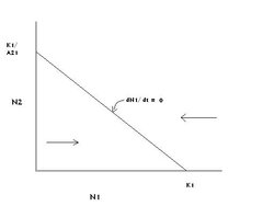 Figure 1: The graph of species 1's zero growth line in competition with species 2. (Source: Carl Hoagstrom, redrawn from many sources)
 For species 1, the graph consists of a horizontal (X) axis containing values for the population size of species 1 (N1) and a vertical (Y) axis with the population size of species 2 (N2) graphed thereon. The equation is a linear equation, therefore the equation of a straight line. The model’s solution is based on the zero growth lines for each species on this graph. Consider species 1 alone, and the conditions that result in dN1/dt = 0. Two points on the line are readily attainable from the equation for population 1’s growth. These are the intercepts of the zero growth line on the X axis where N2 = 0 and N1 = K1; and on the Y axis where N1 = 0, N2 = K1/A21 (Figure 1).
The X intercept zero growth point = K1:N2 = 0 is somewhat intuitive in the context of the equation. If species 1 is at carrying capacity, it will be using up all the resources and there will be none left over to support species 2 (which will therefore be absent), or to support growth in species 1. According to the logistic model for population growth, species 1 can not grow beyond its carrying capacity so = K1:N2 = 0 is an intuitively logical zero growth point as well as one generated by the model. These substitutions into the equation are shown below:
The Y intercept zero growth point is not so intuitive, but it is clearly true within the context of the equation, and the model. Substitutions of these Y axis values into the equation for growth of species 1 are shown below:
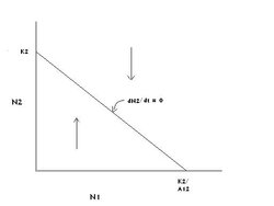 Figure 2: The graph of species 2's zero growth line in competition with species 1. (Source: Carl Hoagstrom, redrawn from many sources)
 The graph in Figure 1 shows the zero growth line for species 1 when competing with species 2 (dN1/dt = 0). Because we have two points and the equation represents a linear relationship, all points on the line drawn between those two points will result in stopping the growth of species 1’s population. All combinations of population sizes (N1 and N2) below the line allow growth (Population growth rate) of species 1‘s population, as indicated by the right-directed arrow. All combinations of population sizes above the line result in a decline of species 1’s population, indicated by the left-directed arrow.
This is an important point for interpretation of the graphs that follow. Any point (represented by a value for N1 and a value for N2, and written N2) on the graph which falls above the zero growth line for a species results in a decline in that population toward the zero growth line. Any point N2 on the graph which falls below a species' zero growth line results in an increase in that population toward the zero growth line.
A similar graph can be generated for species 2’s growth in the face of competition with species 1. Leaving the axes the same (N2 on the Y axis, N1 on the X axis), the graph in Figure 2 is generated. The up and down arrows indicate graphical regions of growth and decline, respectively, of species 2’s population.
The Graphical Solutions of the Lotka-Volterra Competition Model
To solve the two equations and explore competition in the context of the model they represent, both zero growth lines must be placed on the same axes and the interpretation described above must be employed. There are four possible solutions. The model conditions that give rise to the four graphs are described below, and the four graphs are diagrammed alongside the conditions that determine their form.
One Graphical Solution Predicts Competitive Exclusion of Species 2
This solution is generated if K1 > K2/A12 on the X axis; and K1/A21 > K2 on the Y axis (Figure 3).
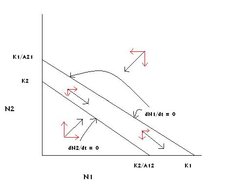 Figure 3: The graphical solution of the Lotka-Volterra competition model in which species 1 competitively excludes species 2. (Source: Carl Hoagstrom, redrawn from many sources)
 Horizontal red arrows indicate growth or decline of population 1 and vertical red arrows indicate growth or decline of population 2 in each region of the graph. The black arrows associated with each pair of red arrows indicate the movement of the two population sizes in that region of the graph.
The arrows indicate that both species’ populations grow in the triangular zone below both zero growth lines.
The arrows show that both species’ populations decline in the zone above both zero growth lines.
In the space between the zero growth lines, above species 2’s and below species 1’s, species 2 must decrease and species 1 will increase, as indicated by the arrows in that region.
Whatever population sizes (N1 and N2 at point [N1:N2]) this two-species community starts with, growth and decline of the two species will continue until the point = K1:N2 = 0 is reached. At that point species 1’s population is at its carrying capacity and species 2’s population is at zero (species 2 is absent). = K1:N2 = 0 is the only stable equilibrium point on the graph. The model concludes that under these conditions, Species 1 will competitively exclude species 2.
Consideration of the prescribed axial relationships lends intuitive credibility to the graphical conclusion:
The environment’s carrying capacity for species 1 is relatively larger than it is for species 2, and species 1 interferes with the growth of species 2 more intensely than species 2 interferes with the growth of species 1. This intuitive conclusion follows because: For K1 > K2/A12, K2 must be relatively small and A12 (in the denominator, and an indicator of the strength of the competition of species 1 on species 2) must be relatively large. The same logic applied to the Y axis gives a relatively small K2 and small A21. The environment has a greater carrying capacity for species 1 than for species 2, and species 1 interferes more with species 2’s growth than species 2 does with species 1’s. Both relationships favor species 1. Species 1 is the superior competitor under these conditions, and species 1 competitively excludes species 2 at equilibrium.
Another Graphical Solution Predicts Competitive Exclusion of Species 1
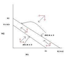 Figure 4: The graphical solution of the Lotka-Volterra competition model in which species 2 competitively excludes species 1. (Source: Carl Hoagstrom, redrawn from many sources)
 Now reverse the axial relationships so that on the X axis K1 < K2/A12 and on the Y axis K1/A21 < K2 (Figure 4).
Parallel logic to that given above gives = 0:N2 = K2 as the only stable equilibrium point, and at equilibrium species 2’s population will be at the environment’s carrying capacity for species 2, while species 1’s population is at zero. Species 2 will competitively exclude species 1.
A Third Graphical Solution Predicts Competitive Exclusion of Species 1 OR 2
Next consider the situation with each carrying capacity having the larger value on its axis, or
On the X axis K1 > K2/A12 and on the Y axis K2 > K1/A21
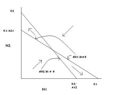 Figure 5: The graphical solution of the Lotka-Volterra competition model in which species 1 or 2 competitively excludes the other species. (Source: Carl Hoagstrom, redrawn from many sources)
 There are three equilibrium points on this graph (Figure 5), but only two are stable equilibrium points, = K1:N2 = 0; and = K2. The point at which the two zero growth lines cross is an unstable equilibrium point. Much of the graph’s area directs the populations to that point, but if perturbed from that point into either adjacent triangle (above and to the left or below and to the right) population sizes will be driven to one of the stable equilibrium points where one species is at its carrying capacity and the other has been competitively excluded. Which species is competitively excluded is often determined by the relative sizes of the initial populations. If there is a large population of species 2 (N2 is large) and a small population of species 1 (N1 is small), the equilibrium result will usually be arrested at = 0:N2 = K2. If the initial population sizes are reversed, the point = K1:N2 = 0 is likely to be achieved at equilibrium.
The Fourth Graphical Solution Predicts the Requirements for Coexistence
Finally, consider the fourth possible solution, both carrying capacities represent the smaller values on their axes, or
On the X axis, K2/A12 > K1 and on the Y axis, K1/A21 > K2
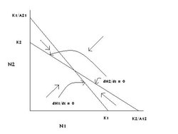 Figure 6: The graphical solution of the Lotka-Volterra competition model in which species 1 and species 2 coexist at equilibrium. (Source: Carl Hoagstrom, redrawn from many sources)
 Whatever the original sizes of the two populations in this graphical space (Figure 6), they will end up at the point where the two zero growth lines intersect. That point is the only stable equilibrium point on the graph and the only stable equilibrium point on all four graphs with both species present (neither N2 nor N1 is zero). In other words, this is the only one of the graphical solutions that results in coexistence of the two species over time. What is special about this solution?
For the terms K1/A21 and K2/A12 to be large (larger than K2 and K1 respectively), the two competition coefficients must be small. They are in the denominator of a large fraction, if denominators are large, fractions will be small. Using the same intuitive logic, in each of the other three solutions (graphs), one or both of the competition coefficients is (are) large. And in each of those cases, one species competitively excludes the other.
Thus the Lotka-Volterra model concludes that species coexist only when competition coefficients are small and thus competition between (or among) the species is minimal.
Testing the Model in the Laboratory
So, the mathematics says that two species that use their resources in ways that are too similar compete too intensely and will not be able to live together indefinitely, but can the model be tested on real species? An endless number of challenges, attempts to refute or support the theory, have been mounted and have resulted in the gathering of much ecological information and understanding. A few of the better known tests of the model are described below.
Georgii F. Gause tested the principle in a laboratory experiment with two species of the aquatic protozoan Paramecium. He placed them both in the same vessel of culture medium with bacteria as their only food source. This situation should result in intense competition because both Paramecium species had only the bacteria as food. If the principle is correct, the population of one Paramecium species should have increased, while the other decreased, eventually decreasing to zero. That was exactly what happened in the experiment. The result that Gause obtained supported the principle. The principle is sometimes called Gause’s law to recognize his experimental contribution.
Thomas Park did the same sort of thing with flour beetles, placing two species in the same vat of flour and monitoring their populations through time. In each experiment the predicted extinction of one species resulted from apparent competition with the other, competitive exclusion. An interesting aspect of Park’s experiments was that he could change the winner of the competition by changing the temperature and humidity of the beetles’ environment. The most important result was that the competitive exclusion principle held: in each case, under a given set of conditions, only one species remained after some time in competition. The other was competitively excluded.
Interestingly, both Gause and Park found situations in which their two experimental species could coexist in the artificial communities they set up. Certain pairs of Gause’s Paramecium species separated in the column of culture medium, one living near the top and the other near the bottom. They could live together in the same culture medium, at different levels; they could coexist if they separated their resource use this way. When Park changed the temperature and humidity periodically, first favoring one species and then the other, his flour beetles could also coexist. Both of these results support the competitive exclusion principle, demonstrating that the way to avoid competitive exclusion is to use the available resources in different ways. Intense competition may result in the weaker competitor being excluded or the competitors may subdivide the available resources so as to minimize overlap in their use. Both results are consistent with the competitive exclusion principle.
Testing the Model in Natural Settings
So, laboratory experiments supported the competitive exclusion principle, but the results might just be artifacts of highly oversimplified systems. Could the principle be tested in the more natural and complex context of ecological communities? A number of experiments and observations have been carried out attempting to answer this challenge. Robert MacArthur’s work with wood warblers is a well known example. He found five species of wood warbler living and raising offspring in the same woods. All fed on insects gleaned from surfaces or caught in flight and in general used resources in ways that seemed very similar, an apparent violation of the competitive exclusion principle. MacArthur watched the warblers carefully and monitored their foraging habits. He found that each species had a unique pattern of foraging in a tree. One foraged primarily at the tops of the trees, another near the ground, others in the middle of the trees, some toward the trunk, others toward the branch tips. He found that their foraging behaviors differed in other ways as well. In other words, the species shared resources, and avoided competitive exclusion, by foraging in different microhabitats and employing different foraging behaviors. Differently stated, each species may have been competitively excluding the others from its foraging microhabitat, thus allowing coexistence in the larger habitat; with the use of different foraging techniques enhancing resource sharing. A large number of similar studies have supported the competitive exclusion principle, though some have seemed to refute it.
More elaborate models have been generated to study competition. Many of them start with the Lotka-Volterra model and build additional complexity into it. Probably all of them trace their roots to Lotka and Volterra, even if they do not build directly on their equations. The importance of competition in community organization has been debated, and much remains unsettled about the conditions under which competitions is more or less important than othe ecological factors in regulating population size and community structure. However, the importance of the competitive exclusion principle in inspiring observational and experimental ecological research, and as a pioneering effort at mathematical modeling in ecology, is widely accepted.
Further Reading
- Colinvaux, Paul. 1978. Why Big Fierce Animals are Rare. Princeton, New Jersey: Princeton University Press. ISBN: 0691023646.
- Gause, G. F. 1934. The Struggle for Existence. Baltimore: Williams and Wilkens. ISBN: 0486495205.
- Gotelli, Nicholas J. 2008. A Primer of Ecology, 4th Edition. Sunderland, Massachusetts: Sinauer Associates, Inc. ISBN: 0878933182.
- Hardin, Garrett. 1960. The Competitive Exclusion Principle. Science 131:1292-1297.
- Competitive Exclusion Principle. Wikipedia.
- Lotka, Alfred J. 1956. Elements of Mathematical Biology. New York: Dover. A reprint with revisions of the original 1925, Elements of Physical Biology. Baltimore: Williams and Wilkens. ISBN: 0486603466.
- Real, Leslie A. and James H. Brown, eds. 1991. Foundations of Ecology: Classic Papers with Commentaries. Chicago: University of Chicago Press. MacArthur’s warbler paper (page 686, published in 1958) and Park’s flour beetle paper (page 754, published in 1948) are reprinted here. The commentaries and several other papers are instructive on the topic of competition. ISBN: 0226705943.