Google Sheets
Modifying Columns, Rows, and Cells
Freezing rows and columns
When working with large spreadsheets, there will be times when you'll want to see certain rows or columns all the time, especially when using header cells as in our example below. By freezing rows or columns in place, you'll be able to scroll through your spreadsheet while continuing to see the header cells.
To freeze a row:
You can freeze up to 10 rows at the top of a spreadsheet.
- Locate the row or rows you wish to freeze. In this example, we will freeze the top two rows.
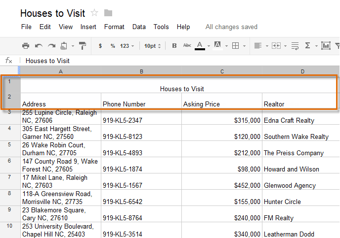 Deciding which rows to freeze
 - Locate and click View in the toolbar menu. Hover the mouse over Freeze rows, then select the desired number of rows to freeze from the drop-down menu.
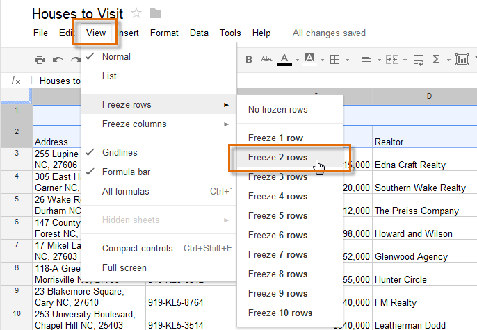 Freezing rows
 - The top two rows are frozen in place. You can scroll down your worksheet while continuing to view the frozen rows at the top.
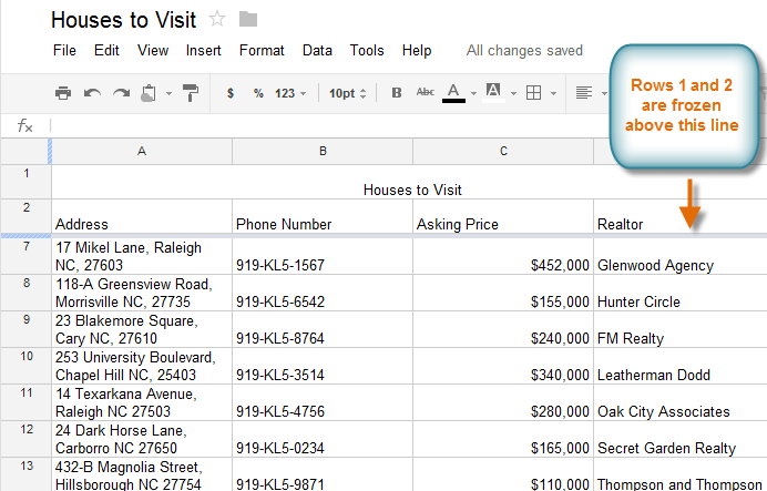 The frozen rows
To freeze a column:
You can freeze up to five columns on the left-hand side of a spreadsheet.
- Locate the column or columns you wish to freeze. In this example, we will freeze the leftmost column.
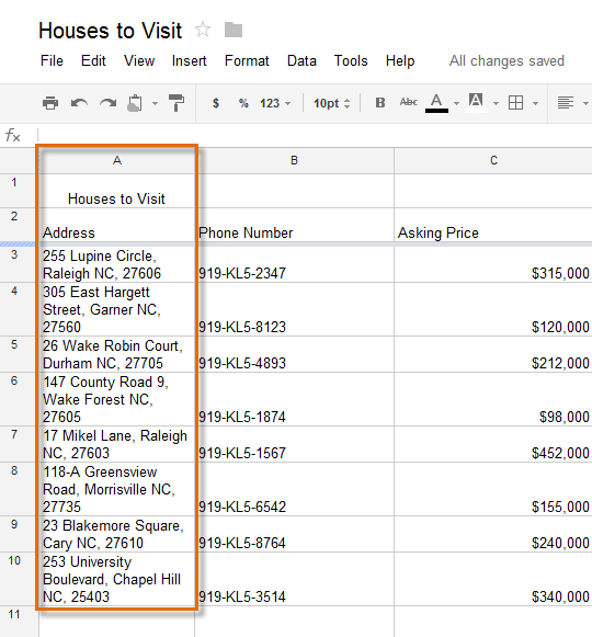 Choosing which column to freeze
 - Locate and click View in the toolbar menu. Hover the mouse over Freeze columns, then select the desired number of columns to freeze from the drop-down menu.
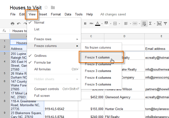 Freezing a column
 - The leftmost column is now frozen in place. You can scroll across your worksheet while continuing to view the frozen column on the left.
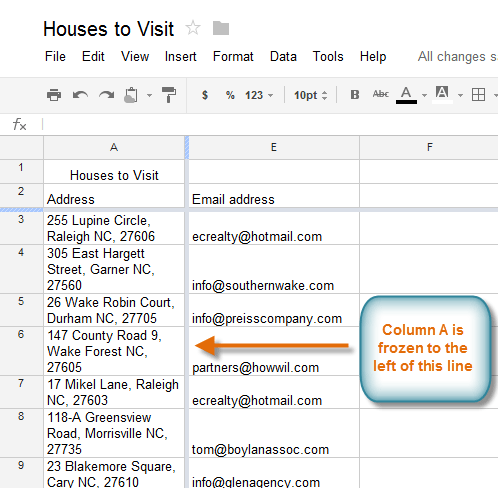 The frozen column
To unfreeze rows, click View in the toolbar menu, hover the mouse over Freeze rows, then select No frozen rows. To unfreeze columns, click View in the toolbar menu, hover the mouse over Freeze columns, then select No frozen columns.
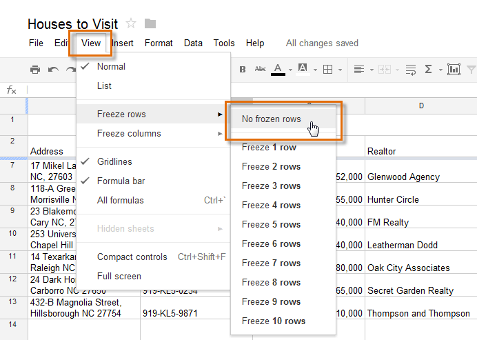 Unfreezing a row


