Regional modeling of the Arctic
This is Section 4.5 of the Arctic Climate Impact Assessment.
Lead Authors: Vladimir M. Kattsov, Erland Källén; Contributing Authors: Howard Cattle, Jens Christensen, Helge Drange, Inger Hanssen-Bauer,Tómas Jóhannesen, Igor Karol, Jouni Räisänen, Gunilla Svensson, Stanislav Vavulin; Consulting Authors: Deliang Chen, Igor Polyakov, Annette Rinke
Contents
Introduction
An improved understanding of the arctic climate system is necessary to provide better quantitative assessments of the magnitude of potential global change and to clarify the role of the Arctic in the global climate system. The deficiencies of AOGCMs (Regional modeling of the Arctic) in describing arctic climate are partly due to inadequate parameterizations of physical processes. Equally important, AOGCMs are characterized by a rather coarse horizontal resolution, which fails to capture atmospheric mesoscale features caused by coastlines, ice sheets, sea-ice margins, and mountains. To some extent, this failure is overcome when the resolution is increased[1]. The most obvious step—to simply increase resolution in AOGCMs—has until now been impractical due to the computational capacities required. Experience with high- or variable-resolution AGCMs has been limited and no results are available that focus on the performance of these models for the Arctic.
Another approach to obtaining enhanced regional details is the use of a nested limited-area model. This technique has garnered considerable interest in recent years because it requires less computational capacity than a global model with comparable resolution. These models can be used for process studies and for model validation studies using lateral boundaries from observation-based analysis[2]. However, the technique can also be used as the basis for dynamic downscaling of AOGCM simulations. Models used in this way are often referred to as regional climate models (RCMs).
Regional climate models of the arctic atmosphere
General
Regional models show considerable skill in short-term (few hour to few day) weather forecasting and are used worldwide for this purpose. This application is basically an initial-value problem, and most of the success of this approach can be ascribed to the high resolution of the models and the use of very recent observations.
Likewise, at timescales of a few years to decades and beyond, regional models have shown their strength in comparison with coarse-resolution global models, as they are capable of capturing the fine-scale details of climatic processes – such as the presence of complex topography and small-scale weather features such as tropical cyclones and even polar lows—much more realistically than global models[3]. Moreover, it has been shown that the statistics of extreme precipitation are realistically simulated by high-resolution regional models[4] and that they show skill even at their grid scale[5]. This is a boundary-value problem and the assessment of the skill of the model is based on statistics of model performance over long time periods (several years or more).
Regional model projections are limited by the quality of the global model projections used for the lateral boundary conditions. In this respect, a potential problem is the mismatch between scales in the coarse-resolution global model and the high-resolution regional model. Recently, this has been demonstrated not to be a fundamental problem if proper boundary condition procedures are used[6]. In fact, it has been demonstrated that, when driven by realistic (observed) boundary conditions, regional climate models are capable of capturing the overall observed regional climatic evolution and can add realistic spatial and temporal information to the information provided by the driving model[7]. When nested within a GCM, it is important, however, to stress that the large scale circulation is imposed by the lateral boundaries. The regional model is not able to, nor is it intended to, correct the large-scale errors made by the global model. The role of the regional model is instead to add regional detail and fine spatial and temporal scales to the simulation, not to improve the large-scale simulation.
Atmospheric regional modeling systems for the Arctic have been developed by Lynch et al.[8] and Dethloff et al.[9]. Dethloff et al.[10] applied the regional atmospheric climate model HIRHAM[11] to the entire Arctic north of 65° N. This model has so far been the only RCM used with a circumpolar focus for climate simulations, although the recent Arctic Regional Model Intercomparison Project (ARCMIP; see Section 4.5.1.2 (Regional modeling of the Arctic)) initiative has increased the interest in arctic RCMs. Many other groups have developed RCMs, but mostly with a more southerly region of interest, although in some cases parts of the Arctic have been included in simulations performed with these models. For example, several models have been applied over most of the European continent including the Scandinavian Peninsula and parts of the North Atlantic Ocean extending all the way to the ice margins; even parts of have been included in such simulations[12]. Likewise, experiments with a Canadian RCM have been applied to the whole of Canada[13] including a fair proportion of the Arctic. The development of these models continues, but limited results with an arctic focus have been published.
Giorgi et al.[14] documented how much insight has been provided into fundamental issues concerning the nested regional modeling technique. For example, multi-year to multi-decadal simulations must be used for climate change studies to provide meaningful climate statistics, to identify significant systematic model errors and climate changes relative to internal model and observed climate variability, and to allow the atmospheric model to equilibrate with the land surface conditions[15]. In addition, the choice of domain size is not a trivial question. The influence of the boundary forcing is reduced as region size increases[16] and may be dominated by the internal model physics for certain variables and seasons[17]. This can lead to the RCM solution significantly departing from the driving data, which can make the interpretation of downscaled regional climate changes more difficult[18]. For most experiments with very high resolution, the domain size is limited by practical considerations and the large-scale flow is, therefore, constrained substantially by the driving model[19]. Denis et al.[20] demonstrated that when the discrepancy in resolution between the model providing the lateral boundary conditions and the nested RCM does not exceed a factor of 10, the RCM is able to generate added value, high-resolution information. With this limitation, they also showed that for a typically sized domain, the RCM does not introduce any spurious developments due to the nesting technique, and is fully capable of a consistent development within the model domain.
Configurations of RCM model physics are derived either from a pre-existing (and well-tested) limited-area model system with modifications suitable for climate applications or are implemented directly from a GCM[21]. In the first approach, each set of parameterizations is developed and optimized for the respective model resolutions. However, this makes interpreting differences between the nested model and the driving GCM more difficult, as these will result from more than just changes in resolution. Also, the different model physics schemes may result in inconsistencies near the boundaries[22]. The second approach maximizes compatibility between the models. However, physics schemes developed for coarse-resolution GCMs may not always be adequate for the high resolutions used in nested regional models and may at a minimum require recalibration. Overall, both strategies have shown performance of similar quality and either is acceptable[23].
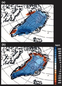 Fig. 4.26. Net mass balance of the Greenland Ice Sheet over the period 1961–1990 simulated by (a) the ECHAM4/OPYC3 general circulation model and (b) the HIRHAM regional climate model. Model-designated elevation contours shown for every 500 m[24].
 Simulations of present-day climate with regional climate models
Regional climate models have been used for a wide variety of research worldwide, and have generated a sizeable research community. However, very few groups have focused on the Arctic to date, although several new initiatives have recently been undertaken. Intercomparison projects entailing participation of different international research groups have been conducted or are currently underway[25]. This section describes the existing applications of RCMs for simulating present-day arctic climate conditions.
Advances in regional climate modeling must be based on an analysis of physical processes and comparison with observations. In data-poor regions such as the Arctic, this procedure may be complemented by a community-based approach (i.e., through collaborative analysis by several research groups). To illustrate this approach, simulations of the Arctic Basin north of 65° N have been performed and planned with different RCMs, driven at their lateral boundaries by observationally based analyses[26]. Motivated by this, an international intercomparison of regional model simulations for the Arctic, ARCMIP, has been organized under the auspices of the World Climate Research Programme. The foci of the evaluation include the surface energy balance over ocean and land, clouds and precipitation processes, stable planetary boundary layer turbulence, ice-albedo feedback, and sea-ice (Sea ice in the Arctic) processes. The preliminary results from this project indicate that the participating regional models are able to reproduce reasonably well the main features of the large-scale flow and the surface parameters in the Arctic. However, in order to reach definitive conclusions in an RCM intercomparison, ensemble simulations with adequate spin-up (time for regional model processes to equilibrate with prescribed external forcings) and equivalent initialization of surface fields are required[27]. Several aspects of the intercomparison are difficult due to the lack of adequate data for model validation. However, some aspects of the models, such as the hydrological cycle, compare well with each other[28].
Determining the primary causes of model biases, deficiencies, and uncertainties in atmosphere-only and coupled atmosphere–ice–ocean climate models for the Arctic is of vital importance in order to model the arctic climate adequately. Participants in the ARCMIP project are seeking to improve model representations through an intercomparison of simulations by different models and comparison with observations made during the Surface Heat Budget of the Arctic Ocean field— experiment year (October 1997 to October 1998).
For the Arctic, only very limited multi-year RCM experiments have been conducted. For example, Kiilsholm et al.[29] assessed the uncertainty in regional accumulation rates for the Greenland Ice Sheet due to model resolution. They used the HIRHAM RCM (50 km resolution) with boundary conditions from a 30-year control simulation with the ECHAM4/OPYC3 model[30] (~300 km horizontal resolution). Figure 4.26 compares the resulting accumulation and ablation zones as simulated by the RCM and the GCM. Table 4.6 illustrates the ability of the models to simulate present regional (northern Greenland) changes in accumulation rates. It appears that the RCM simulation is in better agreement with the observational evidence than the GCM simulation.
|
Table 4.6. Comparison of observed changes in net accumulation rates for the north Greenland Ice Sheet (76°–79° N) with simulations by a general circulation model (ECHAM4/OPYC3) and a regional climate model (HIRHAM). Model uncertainties are estimated as one standard deviation of the 30-year interannual variability in the simulation. | ||
| Change in net accumulation rate (mm/yr) | ||
| 27°–30° W | 60°–65° W | |
|
ECHAM4/OPYC3a |
170±40 | -1390±560 |
|
HIRHAMa |
75±24 | -223±189 |
|
Observedb |
97±84 | -310±107 |
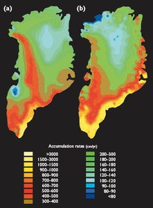 Fig. 4.27. Net accumulation rates over the Greenland Ice Sheet (a) estimated from observations and (b) four years of HIRHAM simulation[33].
 Non-arctic applications have shown that regional models may have significant potential for use as dynamic interpolators, yielding useful data for a wide range of times and locations where in situ observations are not available. As regional models become increasingly accurate, they could become valuable tools for glaciological research. A primary application in glaciology is the investigation of mass balance changes in continental ice sheets. Determining the climatic conditions affecting ice sheets is important because major changes in ice-sheet dimensions affect climate and sea level throughout the world. Much recent work has gone into the validation of RCM simulations[34] using observational data analyses[35] for the Greenland Ice Sheet. Dethloff et al.[36] carried out a detailed RCM validation study on the basis of multi-year ensemble simulations, selected annual simulations, and derived results for the mass balance of the Greenland Ice Sheet. Figure 4.27 illustrates net accumulation rates from the HIRHAM simulations. Compared with available results from earlier work, these results indicate a high degree of skill in spatial representation.
Another promising application was identified by Christensen J. and Kuhry[37], who analyzed the ability of an RCM to simulate permafrost (Permafrost in the Arctic) zonation at very high spatial resolution. Based on a simple permafrost index[38], but applied to the subsurface model layers rather than near-surface air temperatures, they documented that at sufficiently high resolution the permafrost zonation in complex regions can be quite accurately modeled.
Time-slice projections from atmospheric RCMs
In its Third Assessment Report[39] the IPCC considered the concept of using RCMs for climate change projections at some length, and concluded that it is essential that information from a transient AOGCM simulation be available. In such studies, the RCM is used to provide a reinterpretation of the overall AOGCM behavior, including its response to external forcing (from GHGs and aerosols). Sometimes ocean modeling is also done as part of the regional model simulation[40]. In a typical experiment[41], two time slices (e.g., 1961–1990 and 2071–2100) are selected from a transient AOGCM simulation. The RCM simulations include prescribed time-dependent GHG and aerosol concentrations for the corresponding periods of the AOGCM run. The time-dependent sea surface temperatures and sea-ice distributions simulated by the AOGCM are also prescribed as lower boundary conditions, although some models also incorporate an interactive ocean/sea-ice model[42]. The RCM simulations are typically initialized using atmospheric and land-surface conditions interpolated from the corresponding AOGCM fields, and there may be a considerable spin-up period before the actual simulation is started[43].
Only a few studies of this type have been conducted for time slices of durations long enough to encompass the large interannual variability in Arctic. Only two sets of experiments exist to date that cover the entire Arctic[44], while Haugen et al.[45] reported simulations that only cover the Atlantic sector, with the main focus of the experiment being Norwegian land territories (mainland Norway and Svalbard). Kiilsholm et al.[46] and Dorn et al.[47] have conducted a set of such experiments using information from transient simulations with the ECHAM4/OPYC3 model[48].
This section highlights the experiments conducted by Kiilsholm et al.[49] using the HIRHAM4 model forced with the B2 emissions scenario, as they are the only ones with complete multi-year integrations that are generally consistent with the characteristics of the ACIA scenarios. In this study, the AOGCM had a resolution of approximately 300 km, while the resolution of the RCM was approximately 50 km. This discussion focuses on differences in the climate projections of the RCM and the driving AOGCM.
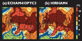 Fig. 4.28. Winter (Dec–Feb) temperature increase in the Arctic between 1961–1990 and 2070–2100 projected by (a) the ECHAM/OPYC3 general circulation model and (b) the HIRHAM4 regional climate model[50].
 Figure 4.28 depicts the winter temperature change as simulated by the AOGCM and the RCM. In general, the patterns of warming as well as their amplitude are quite similar. However, the RCM depicts some regional patterns that can be ascribed to the higher resolution.
Along the ice margin in the Greenland Sea and the Barents Sea, where sea ice (Sea ice in the Arctic) retreats in the simulations (sea ice in the RCM is interpolated from the AOGCM), the RCM shows greater temperature increases. This is due to a stronger response to sea-ice changes resulting from a better description of the nonlinear energy cascade connected with mesoscale weather developments (e.g., stronger cyclonic developments) in the RCM than in the AOGCM. Conversely, temperature increases projected by the RCM tend to be lower over most of the central Arctic and all of Siberia, particularly during summer. This is due to a more realistic simulation of the present-day snow pack by the RCM than by the AOGCM.
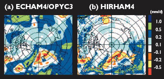 Fig. 4.29. Winter (Dec–Feb) change in precipitation minus evaporation between 1961–1990 and 2070–2100 projected by (a) the ECHAM/OPYC3 general circulation model and (b) the HIRHAM4 regional climate model[51].
 Figure 4.29 shows the winter change in simulated precipitation minus evaporation. As with temperature, the large-scale agreement is striking. However, regional details are evident along the North Atlantic storm track and close to complex topography. In general, the RCM shows a stronger increase in precipitation minus evaporation upwind of major topographical obstacles and a corresponding decrease in precipitation minus evapotranspiration downwind (e.g., Scandinavia, the Rocky Mountains, and Siberia). This is partly explained by the increased topographical gradients due to the higher resolution of the model.
These apparently small differences may have substantial effects on the assessment of future changes in various geophysical systems, such as the mass balance of glaciers and the Greenland Ice Sheet in particular[52] and the depth of the permafrost active layer[53] (Section 6.6 (Regional modeling of the Arctic)). The RCM is better suited for simulating climate change at the regional level, particularly for areas with complex topography and coastlines. This has been confirmed in multiple applications of the model outside of the Arctic[54].
Projected changes in arctic climate due to anthropogenic GHG emissions will occur together with natural dynamic processes in the climate system. In order to improve projections of the evolution of arctic climate, the effects of natural climate variability and in particular their regional dimensions must be taken into account. One major phenomenon contributing to the natural variability of the climate of the Northern Hemisphere is the NAO, which is also associated with the AO, and is described in more detail in Section 2.2.2 (Regional modeling of the Arctic). In general, the influence of the NAO on arctic temperatures is directly opposed in the western and eastern Arctic, and is stronger over land areas than over ocean areas or sea ice. Dorn et al.[55] investigated the combined effects of varying phases of the NAO and increasing GHG and aerosol concentrations on arctic winter temperatures (Fig. 4.30). In this study, different phases of the NAO in a transient coupled AOGCM simulation were considered in time slice simulations using an RCM. Two future periods, 2013–2020 and 2039–2046, representing a positive and a negative phase of the NAO, respectively, were analyzed. The level of GHGs and aerosols in the simulation is higher during the negative NAO phase (2039–2046) than during the positive phase (2013–2020). Although mean arctic winter temperatures are projected to be approximately 1.3 °C higher during the negative phase compared to the positive phase, regions of warming and cooling between the two periods can be observed in Figs. 4.30a and 4.30b. Subsequent to the positive phase, a strong warming of more than 6 °C is simulated over some areas of Alaska (Impacts of global warming in Alaska), the Labrador Sea, and Baffin Island, whereas a similar strong cooling is simulated only over the northern Barents Sea. The temperature effect of the NAO is altered by the general temperature increase resulting from enhanced GHG and aerosol concentrations, but the influence of the NAO is still clearly evident at the regional scale. Although the statistical significance of these differences has not been assessed, the results clearly show that regional changes in the Arctic at decadal timescales may, at least for several more decades, be dominated by changes in the overall atmospheric flow rather than by the temperature increases due to rising GHG concentrations.
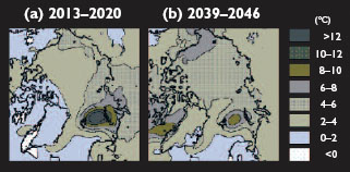 Fig. 4.30. Projected change in monthly mean winter (Dec–Mar) temperature at 2 m height compared to the control climate for (a) 2013–2020, when the simulated North Atlantic Oscillation (NAO) was in a positive phase; and (b) 2039–2046, when the simulated NAO was in a negative phase[56].
 Circulation in an RCM is determined by the boundary conditions provided by the driving AOGCM. As noted in Section 4.3 (Regional modeling of the Arctic), simulations from different global models can be very different in terms of circulation patterns, and the small-scale response in a regional model can amplify such differences. An example is given in Fig. 4.31. Here, the Rossby Centre regional model (RCAO)[57] is driven by 30-year global climate simulations from the HadAM3H and ECHAM4/OPYC3 global climate models forced with the A2 and B2 emissions scenarios. Both regional simulations driven by the HadAM3H scenarios (Fig. 4.31a,b) show only moderate increases in precipitation while both ECHAM4/OPYC3 simulations (Fig. 4.31c,d) show dramatic precipitation increases, particularly on the western side of the Scandinavian mountains. The difference between the A2 and B2 emissions scenarios is quite small relative to the inter-model differences, which are due to a clear difference in the circulation regime change simulated by the two AOGCMs. The HadAM3H model projects a relatively small change in the north-south pressure gradient across the Nordic region, in sharp contrast to the ECHAM4/OPYC3 model, which projects a substantial strengthening of the north–south pressure gradient. This difference is in turn connected with a difference in the projected shifts in the main storm track regions over the North Atlantic. The physical reason behind the different responses in storm track regions for the two global models is at present unclear. Keeping in mind the results of Dorn et al.[58], a plausible explanation is that part of the difference may be due to different simulations of decadal variability in the NAO by the two AOGCMs.
The lack of experiments with different RCMs using boundary conditions from more than one GCM so far prevents the practical use of RCM information for general impacts work. This is also the situation even for better-studied regions, such as continental Europe, due to a lack of appropriate coordination of these efforts; however, see Christensen J. et al.[59] for an update on recent progress.
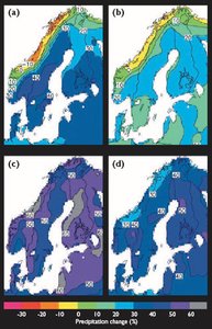 Fig. 4.31. Percentage changes in winter (Dec–Feb) precipitation over the Scandinavian region between 1961–1990 and 2071–2100 as simulated by a regional climate model (RCAO) driven by (a) the HadAM3H model forced with the A2 emissions scenario; (b) the HadAM3H model forced with the B2 emissions scenario; © the ECHAM4/OPYC3 model forced with the A2 emissions scenario; and (d) the ECHAM4/OPYC3 model forced with the B2 emissions scenario.
 Regional Arctic Ocean models
Proper treatment of the Arctic Ocean requires a spatial resolution high enough to account for reduced Rossby length scales (the smallest scale at which the rotation of the Earth has a dominating influence on flow dynamics); to permit the important flows through Bering Strait and the Canadian Archipelago; and to accurately represent the complex bottom topography steering the currents, as well as the continental slopes and the large continental shelves where the thermohaline, wind-driven, and tidal dynamics interact.
Currently, about a dozen Arctic Ocean models exist, most of which are participating in the Arctic Ocean Model Intercomparison Project (AOMIP)[60]. Most of the Arctic Ocean models are derived from global oceanic GCMs – in many cases from the Geophysical Fluid Dynamics Laboratory (GFDL) Modular Ocean Model (MOM)[61]. The Arctic Ocean models represent a wide spectrum of numerical approaches, employing either finite-difference (in most cases) or finite-element approximations, and three types of vertical coordinates: z (constant geopotential surfaces), sigma (bathymetry-following), and isopycnal (constant potential density referenced to a given pressure). The models differ in their spatial resolution (from 40–50 km down to 16–20 km in the horizontal and typically 25–30 levels in the vertical); specifications of surface and lateral fluxes; and formulations of the surface mixed and bottom boundary layers. Regional models of the Arctic Ocean are usually coupled to comprehensive sea-ice models, although these often differ in their treatment of dynamics and thermodynamics.
To ensure a degree of fidelity to the simulations, an artificial constraint known as "climate restoring" (i.e., relaxation to the observed climate) based on the surface salinity is often introduced. This constraint prevents a model from drifting significantly from observations. Restoring time constants vary across models from several months (strong restoring) to several years (weak restoring). Some models do not employ restoring at all. However, the biases in simulations monotonically increase with the value of the restoring constant, reaching their highest levels in the models without restoring[62]. This emphasizes that there are some processes and feedbacks crucial for representing the Arctic Ocean general circulation that are still neither sufficiently understood nor properly represented in the regional models, just as is the case for the global models.
From the viewpoint of their employment in downscaling AOGCM outputs or in constructing scenarios of future climate change, regional ocean models lag behind the atmospheric RCMs.
Coupled arctic regional climate models
The construction of coupled RCMs is a recent development. These models couple atmospheric RCMs to other models of climate system components, such as lake, ocean/sea-ice, chemistry/aerosol, and land biosphere/ hydrology models[63]. These initial efforts provide a path toward the development of coupled "regional climate system models". For some parts of the Arctic, coupled mesoscale atmosphere–ice–ocean models already exist, although they are restricted to small domains and short integration times[64].
For the circumpolar Arctic, Maslanik et al.[65] presented the first results of a coupled atmosphere–ice–ocean RCM called ARCSyM. The oceanic component in this RCM was a simple mixed layer model. Rinke et al.[66] presented a more complex coupled RCM (i.e., a fully coupled atmosphere–ice–ocean circulation model system) called HIRHAM-MOM. The ability to simulate conditions over the Arctic Ocean during April to September 1990, a period of anomalous atmospheric circulation and sea-ice conditions, was investigated with both models. A common result was found: neither model was able to correctly reproduce the large retreat of sea ice in the eastern Eurasian Basin and the adjacent shelf sea observed during the summer of 1990[67]. The sea ice in the Chukchi and East Siberian Seas does not retreat as completely in the model simulations as it does in observations inferred from satellite data.
The HIRHAM-MOM coupled model[68] reproduced the general sea-level pressure patterns for the summer of 1990, based on a comparison with ECMWF analyses. However, discrepancies appeared in late summer that significantly affected variables such as wind flow and sea-ice transport. Similar to the ARCSyM results[69], HIRHAMMOM simulated too much sea ice in the Bering, Chukchi, and East Siberian Seas during the summer of 1990. This is also the case for the ocean/sea-ice models driven by ECMWF atmospheric data.
The results from both coupled models highlight the importance of regional atmospheric circulation in driving interannual variations in arctic sea-ice extent, and illustrate the level of model performance required to simulate such variations. Such studies are valuable because they indicate improvements needed in the models by evaluating the results against observations, and the roles of key processes and feedbacks by comparing the results to those of the uncoupled atmospheric model. While results for the Baltic Sea imply improved model performance when an ocean model is coupled to the RCM[70], high-resolution coupled model systems for the Arctic have not provided improved performance to date.
Summary
The current status of arctic regional climate modeling did not allow RCMs to be employed as principal tools for the ACIA (Arctic Climate Impact Assessment (ACIA)). Present scenarios of future arctic climate change are therefore based on results from global AOGCMs. However, presently available global coupled models have a coarse spatial resolution that limits their ability to capture many important aspects of climate change. In particular, intense storms, the effects of topography, and fundamental aspects of regional ocean circulation cannot be represented adequately. To improve the modeling of such phenomena, development of regional coupled ocean-ice-atmosphere climate models should receive a high priority in the efforts of the climate modeling community. Such developments should go hand in hand with developments in global modeling, in particular development of high-resolution AOGCMs.
Chapter 4: Future Climate Change: Modeling and Scenarios for the Arctic
4.1. Introduction (Regional modeling of the Arctic)
4.2. Global coupled atmosphere-ocean general circulation models
4.3. Simulation of observed arctic climate with the ACIA designated models
4.4. Arctic climate change scenarios for the 21st century projected by the ACIA-designated models
4.5. Regional modeling of the Arctic
4.6. Statistical downscaling approach and downscaling of AOGCM climate change projections
4.7. Outlook for improving climate change projections for the Arctic
References
Citation
Committee, I. (2012). Regional modeling of the Arctic. Retrieved from http://editors.eol.org/eoearth/wiki/Regional_modeling_of_the_Arctic- ↑ Giorgi, F., B. Hewitson, J. Christensen, M. Hulme, H. von Storch, P. Whetton, R. Jones, L. Mearns and C. Fu, 2001. Regional climate information – evaluation and projections. In: J.T. Houghton, Y. Ding, D.J. Griggs, M. Noguer, P.J. van der Linden, X. Dai, K. Maskell and C.A. Johnson (eds.). pp. 583–638. Climate Change 2001: The Scientific Basis. Contribution of Working Group I to the Third Assessment Report of the Intergovernmental Panel on Climate Change. Cambridge University Press.
- ↑ Giorgi, F. and L.O. Mearns, 1999. Introduction to special section: Regional climate modeling revisited. Journal of Geophysical Research, 104:6335–6352.–Giorgi, F., B. Hewitson, J. Christensen, M. Hulme, H. von Storch, P. Whetton, R. Jones, L. Mearns and C. Fu, 2001. Regional climate information – evaluation and projections. In: J.T. Houghton, Y. Ding, D.J. Griggs, M. Noguer, P.J. van der Linden, X. Dai, K. Maskell and C.A. Johnson (eds.). pp. 583–638. Climate Change 2001: The Scientific Basis. Contribution of Working Group I to the Third Assessment Report of the Intergovernmental Panel on Climate Change. Cambridge University Press.
- ↑ Giorgi, F., B. Hewitson, J. Christensen, M. Hulme, H. von Storch, P. Whetton, R. Jones, L. Mearns and C. Fu, 2001. Regional climate information – evaluation and projections. In: J.T. Houghton, Y. Ding, D.J. Griggs, M. Noguer, P.J. van der Linden, X. Dai, K. Maskell and C.A. Johnson (eds.). pp. 583–638. Climate Change 2001: The Scientific Basis. Contribution of Working Group I to the Third Assessment Report of the Intergovernmental Panel on Climate Change. Cambridge University Press.
- ↑ Frei, C., J.H. Christensen, M. Deque, D. Jacob, R.G. Jones and P.L. Vidale, 2003b. Daily precipitation statistics in regional climate models: evaluation and intercomparison for the European Alps. Journal of Geophysical Research, 108: 10.1029/2002JD002287.
- ↑ Huntingford, C., R.G. Jones, C. Prudhomme, R. Lamb and J.H.C. Gash, 2003. Regional climate model predictions of extreme rainfall for a changing climate. Quarterly Journal of the Royal Meteorological Society, 129:1607–1621.
- ↑ Denis, B., R. Laprise and D. Cava, 2002. Downscaling ability of one-way nested regional climate models: the big-brother experiment. Climate Dynamics, 18:627–646.
- ↑ Dethloff, K., M. Schwager, J.H. Christensen, S. Kiilsholm, A. Rinke, W. Dorn, F. Jung-Rothenhäusler, H. Fischer, S. Kipfstuhl and H. Miller, 2002. Greenland precipitation from ice core estimates and regional climate model simulations. Journal of Climate, 15:2821–2832.–Frei, C., J.H. Christensen, M. Deque, D. Jacob, R.G. Jones and P.L. Vidale, 2003b. Daily precipitation statistics in regional climate models: evaluation and intercomparison for the European Alps. Journal of Geophysical Research, 108: 10.1029/2002JD002287.–Giorgi, F., B. Hewitson, J. Christensen, M. Hulme, H. von Storch, P. Whetton, R. Jones, L. Mearns and C. Fu, 2001. Regional climate information – evaluation and projections. In: J.T. Houghton, Y. Ding, D.J. Griggs, M. Noguer, P.J. van der Linden, X. Dai, K. Maskell and C.A. Johnson (eds.). pp. 583–638. Climate Change 2001: The Scientific Basis. Contribution of Working Group I to the Third Assessment Report of the Intergovernmental Panel on Climate Change. Cambridge University Press.
- ↑ Lynch, A.H., W.L. Chapman, J.E. Walsh and G. Weller, 1995. Development of a regional climate model of the western Arctic. Journal of Climate, 8:1555–1570.
- ↑ Dethloff, K., A. Rinke, R. Lehmann, J.H. Christensen, M. Botzet and B. Machenhauer, 1996. A regional climate model of the Arctic atmosphere. Journal of Geophysical Research, 101:23401–23422.
- ↑ Dethloff, K., A. Rinke, R. Lehmann, J.H. Christensen, M. Botzet and B. Machenhauer, 1996. A regional climate model of the Arctic atmosphere. Journal of Geophysical Research, 101:23401–23422.
- ↑ Christensen, J.H., O.B. Christensen, P. Lopez, E. van Meijgaard and M. Botzet, 1996. The HIRHAM4 Regional Atmospheric Climate Model. Danish Meteorological Institute, Scientific Report 96-4.
- ↑ Christensen, J.H., B. Machenhauer, R.G. Jones, C. Schär, P.M. Ruti, M. Castro and G.Visconti, 1997. Validation of present-day regional climate simulations over Europe: LAM simulations with observed boundary conditions. Climate Dynamics, 13:489–506.–Rummukainen, M., J. Räisänen, B. Bringfelt, A. Ullerstig, A. Omstedt, U. Willén, U. Hansson and C. Jones, 2001. A regional climate model for northern Europe: model description and results from the downscaling of two GCM control simulations. Climate Dynamics, 17:339–359.
- ↑ Laprise, R., D. Caya, M. Giguère, G. Bergeron, H. Côte, J.-P. Blanchet, G.J. Boer and N.A. McFarlane, 1998. Climate and climate change in western Canada as simulated by the Canadian regional climate model. Atmosphere-Ocean, 36:119–167.
- ↑ Giorgi, F., B. Hewitson, J. Christensen, M. Hulme, H. von Storch, P. Whetton, R. Jones, L. Mearns and C. Fu, 2001. Regional climate information – evaluation and projections. In: J.T. Houghton, Y. Ding, D.J. Griggs, M. Noguer, P.J. van der Linden, X. Dai, K. Maskell and C.A. Johnson (eds.). pp. 583–638. Climate Change 2001: The Scientific Basis. Contribution of Working Group I to the Third Assessment Report of the Intergovernmental Panel on Climate Change. Cambridge University Press.
- ↑ Christensen, O.B., 1999. Relaxation of soil variables in a Regional Climate Model. Tellus, 51A:674–685.–Jones, R.G., J.M. Murphy, M. Noguer and A.B. Keen, 1997. Simulation of climate change over Europe using a nested regionalclimate model. II: comparison of driving and regional model responses to a doubling of carbon dioxide. Quarterly Journal of the Royal Meteorological Society, 123:265–292.–Machenhauer, B., J. Windelband, M. Botzet, J.H. Christensen, M. Deque, R. Jones, P.M. Ruti and G. Visconti, 1998. Validation and analysis of regional present-day climate and climate change simulations over Europe. MPI Report 275. Max Planck Institute for meteorology, Hamburg.–McGregor, J.L., J.J. Katzfey and K.C. Nguyen, 1999. Recent regional climate modelling experiments at CSIRO. In: H. Ritchie (ed.). Research Activities in Atmospheric and Oceanic Modelling, pp. 7.37–7.38. CAS/JSC Working Group on Numerical Experimentation Report 28.WMO/TD - No. 942. World Meteorological Organization, Geneva.
- ↑ Jacob, D. and R. Podzun, 1997. Sensitivity studies with the Regional Climate Model REMO. Meteorology and Atmospheric Physics, 63:119–129.–Jones, R.G., J.M. Murphy and M. Noguer, 1995. Simulation of climate change over Europe using a nested regional climate model. I: Assessment of control climate, including sensitivity to location of lateral boundaries. Quarterly Journal of the Royal Meteorological Society, 121:1413–1449.
- ↑ Noguer, M., R. Jones and J. Murphy, 1998. Sources of systematic errors in the climatology of a regional climate model over Europe. Climate Dynamics, 14:691–712.
- ↑ Jones, R.G., J.M. Murphy, M. Noguer and A.B. Keen, 1997. Simulation of climate change over Europe using a nested regionalclimate model. II: comparison of driving and regional model responses to a doubling of carbon dioxide. Quarterly Journal of the Royal Meteorological Society, 123:265–292.
- ↑ Christensen, J.H. and P. Kuhry, 2000. High resolution regional climate model validation and permafrost simulation for the East- European Russian Arctic. Journal of Geophysical Research, 105:29647–29658.
- ↑ Denis, B., R. Laprise and D. Cava, 2002. Downscaling ability of one-way nested regional climate models: the big-brother experiment. Climate Dynamics, 18:627–646.
- ↑ Giorgi, F., B. Hewitson, J. Christensen, M. Hulme, H. von Storch, P. Whetton, R. Jones, L. Mearns and C. Fu, 2001. Regional climate information – evaluation and projections. In: J.T. Houghton, Y. Ding, D.J. Griggs, M. Noguer, P.J. van der Linden, X. Dai, K. Maskell and C.A. Johnson (eds.). pp. 583–638. Climate Change 2001: The Scientific Basis. Contribution of Working Group I to the Third Assessment Report of the Intergovernmental Panel on Climate Change. Cambridge University Press.
- ↑ Machenhauer, B., J. Windelband, M. Botzet, J.H. Christensen, M. Deque, R. Jones, P.M. Ruti and G. Visconti, 1998. Validation and analysis of regional present-day climate and climate change simulations over Europe. MPI Report 275. Max Planck Institute for meteorology, Hamburg.–Rummukainen, M., J. Räisänen, B. Bringfelt, A. Ullerstig, A. Omstedt, U. Willén, U. Hansson and C. Jones, 2001. A regional climate model for northern Europe: model description and results from the downscaling of two GCM control simulations. Climate Dynamics, 17:339–359.
- ↑ Giorgi, F. and L.O. Mearns, 1999. Introduction to special section: Regional climate modeling revisited. Journal of Geophysical Research, 104:6335–6352.
- ↑ Kiilsholm, S., J.H. Christensen, K. Dethloff and A. Rinke, 2003. Net accumulation of the Greenland Ice Sheet: Modelling Arctic regional climate change. Geophysical Research Letters, 30, 10.1029/2002GL015742.
- ↑ Christensen, J.H., B. Machenhauer, R.G. Jones, C. Schär, P.M. Ruti, M. Castro and G.Visconti, 1997. Validation of present-day regional climate simulations over Europe: LAM simulations with observed boundary conditions. Climate Dynamics, 13:489–506.–Christensen, J.H., T.R. Carter and F. Giorgi, 2002. PRUDENCE employs new methods to assess European climate change. Eos, Transactions, American Geophysical Union, 83(13):147.–Machenhauer, B., J. Windelband, M. Botzet, J.H. Christensen, M. Deque, R. Jones, P.M. Ruti and G. Visconti, 1998. Validation and analysis of regional present-day climate and climate change simulations over Europe. MPI Report 275. Max Planck Institute for meteorology, Hamburg.–Takle, E.S., W.J. Gutowski, R.W. Arritt, Z. Pan, C.J. Anderson, R.S. da Silva, D. Caya, S.-C. Chen, F. Giorgi, J.H. Christensen, S.-Y. Hong, H.-M.H. Juang, J. Katzfey, W.M. Lapenta, R. Laprise, P. Lopez, G.E. Liston, J. McGregor, A. Pielke and J.O. Roads, 1999. Project to intercompare regional climate simulation (PIRCS): Description and initial results. Journal of Geophysical Research, 104:19443–19461.–Rinke, A., A.H. Lynch and K. Dethloff, 2000. Intercomparison of Arctic regional climate simulations: case studies of January and June 1990. Journal of Geophysical Research, 105:29669–29683.
- ↑ Rinke, A., A.H. Lynch and K. Dethloff, 2000. Intercomparison of Arctic regional climate simulations: case studies of January and June 1990. Journal of Geophysical Research, 105:29669–29683.
- ↑ Rinke, A., A.H. Lynch and K. Dethloff, 2000. Intercomparison of Arctic regional climate simulations: case studies of January and June 1990. Journal of Geophysical Research, 105:29669–29683.
- ↑ Rinke, A., A.H. Lynch and K. Dethloff, 2000. Intercomparison of Arctic regional climate simulations: case studies of January and June 1990. Journal of Geophysical Research, 105:29669–29683.
- ↑ Kiilsholm, S., J.H. Christensen, K. Dethloff and A. Rinke, 2003. Net accumulation of the Greenland Ice Sheet: Modelling Arctic regional climate change. Geophysical Research Letters, 30, 10.1029/2002GL015742.
- ↑ Roeckner, E., J.M. Oberhuber, A. Bacher, M. Christoph and I. Kirchner, 1996. ENSO variability and atmospheric response in a global coupled atmosphere-ocean GCM. Climate Dynamics, 12:737–754.
- ↑ Kiilsholm, S., J.H. Christensen, K. Dethloff and A. Rinke, 2003. Net accumulation of the Greenland Ice Sheet: Modelling Arctic regional climate change. Geophysical Research Letters, 30, 10.1029/2002GL015742.
- ↑ Paterson, A.B. and N. Reeh, 2001. Thinning of the ice sheet in northwest Greenland over the past forty years. Nature, 414:60–62.
- ↑ Dethloff, K., M. Schwager, J.H. Christensen, S. Kiilsholm, A. Rinke, W. Dorn, F. Jung-Rothenhäusler, H. Fischer, S. Kipfstuhl and H. Miller, 2002. Greenland precipitation from ice core estimates and regional climate model simulations. Journal of Climate, 15:2821–2832.
- ↑ Bromwich, D., J. Cassano, T. Klein, G. Heinemann, K. Hines, K. Steffen and J. Box, 2001. Mesoscale modeling of katabatic winds over Greenland with the Polar MM5. Monthly Weather Review, 129(9):2290–2309.–Cassano, J.J., T.R. Parish and J. King, 2001. Evaluation of turbulent surface flux parameterizations for the stable boundary layer over Halley, Antarctica. Monthly Weather Review, 129:26–46.
- ↑ Hanna, E. and P. Valdes, 2001. Validation of ECMWF (re)analysis surface climate data, 1979–1998 for Greenland and implications for mass balance modelling of the ice sheet. International Journal of Climatology, 21(2):171–195.
- ↑ Dethloff, K., M. Schwager, J.H. Christensen, S. Kiilsholm, A. Rinke, W. Dorn, F. Jung-Rothenhäusler, H. Fischer, S. Kipfstuhl and H. Miller, 2002. Greenland precipitation from ice core estimates and regional climate model simulations. Journal of Climate, 15:2821–2832.
- ↑ Christensen, J.H. and P. Kuhry, 2000. High resolution regional climate model validation and permafrost simulation for the East- European Russian Arctic. Journal of Geophysical Research, 105:29647–29658.
- ↑ Nelson, F.E. and S.I. Outcalt, 1987. A computational method for prediction and regionalization of permafrost. Arctic and Alpine Research, 19:279–288.
- ↑ IPCC, 2001. Climate Change 2001: The Scientific Basis. Contribution of Working Group I to the Third Assessment Report of the Intergovernmental Panel on Climate Change. J.T. Houghton, Y. Ding, D.J. Griggs, M. Noguer, P.J. van der Linden, X. Dai, K. Maskell and C.A. Johnson (eds.). Intergovernmental Panel on Climate Change. Cambridge University Press, 881pp.
- ↑ Räisänen, J., U. Hansson, A. Ullerstig, R. Döscher, L.P. Graham, C. Jones, M. Meier, P. Samuelsson and U. Willén, 2003. GCM driven simulations of recent and future climate with the Rossby Centre coupled atmosphere Baltic Sea regional climate model RCAO. Reports on Meteorology and Climatology, No. 101, Swedish Meteorological and Hydrological Institute, 61pp.
- ↑ Christensen, J.H., T.R. Carter and F. Giorgi, 2002. PRUDENCE employs new methods to assess European climate change. Eos, Transactions, American Geophysical Union, 83(13):147.–Jones, R.G., J.M. Murphy and M. Noguer, 1995. Simulation of climate change over Europe using a nested regional climate model. I: Assessment of control climate, including sensitivity to location of lateral boundaries. Quarterly Journal of the Royal Meteorological Society, 121:1413–1449.–Kiilsholm, S., J.H. Christensen, K. Dethloff and A. Rinke, 2003. Net accumulation of the Greenland Ice Sheet: Modelling Arctic regional climate change. Geophysical Research Letters, 30, 10.1029/2002GL015742.–Machenhauer, B., M. Windelband, M. Botzet, R. Jones and M. Deque, 1996. Validation of present-day regional climate simulations over Europe: Nested LAM and variable resolution global model simulations with observed or mixed layer ocean boundary conditions. MPI Report 191. Max Planck Institute for meteorology, Hamburg.–Räisänen, J., M. Rummukainen, A. Ullerstig, B. Bringfelt, U. Hansson and U. Willén, 1999. The first Rossby Centre regional climate scenario – dynamical downscaling of CO2-induced climate change in the HadCM2 GCM. Reports on Meteorology and Climatology, No. 85, Swedish Meteorological and Hydrological Institute, 56pp.–Rummukainen, M., J. Räisänen, B. Bringfelt, A. Ullerstig, A. Omstedt, U. Willén, U. Hansson and C. Jones, 2001. A regional climate model for northern Europe: model description and results from the downscaling of two GCM control simulations. Climate Dynamics, 17:339–359.
- ↑ Räisänen, J., U. Hansson, A. Ullerstig, R. Döscher, L.P. Graham, C. Jones, M. Meier, P. Samuelsson and U. Willén, 2003. GCM driven simulations of recent and future climate with the Rossby Centre coupled atmosphere Baltic Sea regional climate model RCAO. Reports on Meteorology and Climatology, No. 101, Swedish Meteorological and Hydrological Institute, 61pp.
- ↑ Christensen, O.B., 1999. Relaxation of soil variables in a Regional Climate Model. Tellus, 51A:674–685.
- ↑ Dorn, W., K. Dethloff, A. Rinke and E. Roeckner, 2003. Competition of NAO regime changes and increasing greenhouse gases and aerosols with respect to Arctic climate projections. Climate Dynamics, 21(5–6): 447–458.–Kiilsholm, S., J.H. Christensen, K. Dethloff and A. Rinke, 2003. Net accumulation of the Greenland Ice Sheet: Modelling Arctic regional climate change. Geophysical Research Letters, 30, 10.1029/2002GL015742.
- ↑ Haugen, J.E., D. Bjørge and T.E. Nordeng, 2000. Dynamic downscaling: further results. RegClim General Technical Report, No.4. Available from the Norwegian Institute for Air Research.
- ↑ Kiilsholm, S., J.H. Christensen, K. Dethloff and A. Rinke, 2003. Net accumulation of the Greenland Ice Sheet: Modelling Arctic regional climate change. Geophysical Research Letters, 30, 10.1029/2002GL015742.
- ↑ Dorn, W., K. Dethloff, A. Rinke and E. Roeckner, 2003. Competition of NAO regime changes and increasing greenhouse gases and aerosols with respect to Arctic climate projections. Climate Dynamics, 21(5–6): 447–458.
- ↑ Stendel, M., T. Schmith, E. Roeckner and U. Cubasch, 2000. The climate of the 21st century: transient simulations with a coupled atmosphere-ocean general circulation model. Danish Climate Centre Report 00-6, 51pp.
- ↑ Kiilsholm, S., J.H. Christensen, K. Dethloff and A. Rinke, 2003. Net accumulation of the Greenland Ice Sheet: Modelling Arctic regional climate change. Geophysical Research Letters, 30, 10.1029/2002GL015742.
- ↑ Rysgaard, S., T. Vang, M. Stjernholm, B. Rasmussen, A. Windelin and S. Kiilsholm, 2003. Physical conditions, carbon transport and climate change impacts in a NE Greenland fjord. Arctic, Antarctic and Alpine Research, 35(3):301–312.
- ↑ Ibid.
- ↑ Kiilsholm, S., J.H. Christensen, K. Dethloff and A. Rinke, 2003. Net accumulation of the Greenland Ice Sheet: Modelling Arctic regional climate change. Geophysical Research Letters, 30, 10.1029/2002GL015742.
- ↑ Walsh, J.E., in press. Summary of a workshop on modeling the Arctic atmosphere, Madison, Wisconsin, 20–22 May 2002. Bulletin of the American Meteorological Society.
- ↑ Giorgi, F., B. Hewitson, J. Christensen, M. Hulme, H. von Storch, P. Whetton, R. Jones, L. Mearns and C. Fu, 2001. Regional climate information – evaluation and projections. In: J.T. Houghton, Y. Ding, D.J. Griggs, M. Noguer, P.J. van der Linden, X. Dai, K. Maskell and C.A. Johnson (eds.). pp. 583–638. Climate Change 2001: The Scientific Basis. Contribution of Working Group I to the Third Assessment Report of the Intergovernmental Panel on Climate Change. Cambridge University Press.–Christensen, J.H. and O.B. Christensen, 2003. Severe summer flooding in Europe. Nature, 421:805–806.–Huntingford, C., R.G. Jones, C. Prudhomme, R. Lamb and J.H.C. Gash, 2003. Regional climate model predictions of extreme rainfall for a changing climate. Quarterly Journal of the Royal Meteorological Society, 129:1607–1621.
- ↑ Dorn, W., K. Dethloff, A. Rinke and E. Roeckner, 2003. Competition of NAO regime changes and increasing greenhouse gases and aerosols with respect to Arctic climate projections. Climate Dynamics, 21(5–6): 447–458.
- ↑ Dorn, W., K. Dethloff, A. Rinke and E. Roeckner, 2003. Competition of NAO regime changes and increasing greenhouse gases and aerosols with respect to Arctic climate projections. Climate Dynamics, 21(5–6): 447–458.
- ↑ Rummukainen, M., J. Räisänen, B. Bringfelt, A. Ullerstig, A. Omstedt, U. Willén, U. Hansson and C. Jones, 2001. A regional climate model for northern Europe: model description and results from the downscaling of two GCM control simulations. Climate Dynamics, 17:339–359.
- ↑ Dorn, W., K. Dethloff, A. Rinke and E. Roeckner, 2003. Competition of NAO regime changes and increasing greenhouse gases and aerosols with respect to Arctic climate projections. Climate Dynamics, 21(5–6): 447–458.
- ↑ Christensen, J.H., T.R. Carter and F. Giorgi, 2002. PRUDENCE employs new methods to assess European climate change. Eos, Transactions, American Geophysical Union, 83(13):147.
- ↑ Proshutinsky, A., M. Steele, J. Zhang, G. Holloway, N. Steiner, S. Hakkinen, D. Holland, R. Gerdes, C. Koeberle, M. Karcher, M. Johnson, W. Maslowski, W. Walczowski, W. Hibler and J. Wang, 2001. Multinational effort studies differences among Arctic Ocean models. Eos,Transactions, American Geophysical Union, 82(637):643–644.
- ↑ Pacanowski, R.C. and S.M. Griffies, 1999. The MOM 3 Manual. Geophysical Fluid Dynamics Laboratory/NOAA, Princeton, New Jersey, 680pp.
- ↑ Proshutinsky, A., M. Steele, J. Zhang, G. Holloway, N. Steiner, S. Hakkinen, D. Holland, R. Gerdes, C. Koeberle, M. Karcher, M. Johnson, W. Maslowski, W. Walczowski, W. Hibler and J. Wang, 2001. Multinational effort studies differences among Arctic Ocean models. Eos,Transactions, American Geophysical Union, 82(637):643–644.
- ↑ Bailey, D.A. and A.H. Lynch, 2000a. Development of an Antarctic Regional Climate System Model: Part 1. Sea ice and large-scale circulation. Journal of Climate, 13:1337–1350.–Bailey, D.A. and A.H. Lynch, 2000b. Development of an Antarctic Regional Climate System Model: Part 2. Station validation and surface energy balance. Journal of Climate, 13:1351–1361.–Bailey, D.A., A.H. Lynch and K.S. Hedström, 1997. The impact of ocean circulation on regional polar climate simulations using the Arctic Region Climate System Model. Annals of Glaciology, 25:203–207.–Hostetler, S.W., F. Giorgi, G.T. Bates and P.J. Bartlein, 1994. Lake-atmosphere feedbacks associated with paleolakes Bonneville and Lahontan. Science, 263:665–668.–Lynch, A.H., W.L. Chapman, J.E. Walsh and G. Weller, 1995. Development of a regional climate model of the western Arctic. Journal of Climate, 8:1555–1570.–Lynch, A.H., M.F. Glück, W.L. Chapman, D.A. Bailey and J.E. Walsh, 1997. Remote sensing and climate modeling of the St. Lawrence Is. Polynya. Tellus, 49A:277–297.–Lynch, A.H., D.L. McGinnes and D.A. Bailey, 1998. Snow-albedo and the spring transition in a regional climate system model: influence of land surface model. Journal of Geophysical Research, 103:29037–29049.–Mabuchi, K.,Y. Sato and H. Kida, 2000. Numerical study of the relationships between climate and the carbon dioxide cycle on a regional scale. Journal of the Meteorological Society of Japan, 78:25–46.–Maslanik, J.A., A.H. Lynch, M.C. Serreze and W. Wu, 2000. A case study of regional climate anomalies in the Arctic: performance requirements for a coupled model. Journal of Climate, 13:383–401.–Qian, Y. and F. Giorgi, 1999. Interactive coupling of regional climate and sulfate aerosol models over East Asia. Journal of Geophysical Research, 104:6501–6514.–Rinke, A., R. Gerdes, K. Dethloff, T. Kandlbinder, M. Karcher, F. Kauker, S. Frickenhaus, C. Köberle and W. Hiller, 2003. A case study of the anomalous Arctic sea ice conditions during 1990: insight from coupled and uncoupled regional climate model simulations. Journal of Geophysical Research, 108 (D9),4275, doi:10.1029/2002JD003146.–Roed, L.P., X.B. Shi and B. Hackett, 2000. The Importance of Allowing Turbulent and Diffusive Diapycnal Mixing in Isopycnic Coordinate Ocean Models. RegClim General Tech. Rep. 4, 139–148. Available from the Norwegian Institute for Air Research.–Rummukainen, M., J. Räisänen, B. Bringfelt, A. Ullerstig, A. Omstedt, U. Willén, U. Hansson and C. Jones, 2001. A regional climate model for northern Europe: model description and results from the downscaling of two GCM control simulations. Climate Dynamics, 17:339–359.–Small, E.E., F. Giorgi and L.C. Sloan, 1999a. Regional climate model simulation of precipitation in central Asia: Mean and interannual variability. Journal of Geophysical Research, 104:6563–6582.–Small, E.E., L.C. Sloan, S. Hostetler and F. Giorgi, 1999b. Simulating the water balance of the Aral Sea with a coupled regional climatelake model. Journal of Geophysical Research, 104:6583–6602.–Tsvetsinskaya, E., L.O. Mearns and W.E. Easterling, 2000. Effects of plant growth and development on interannual variability in mesoscale atmospheric simulations. In: Proceedings of the Tenth International Offshore and Polar Engineering Conference.Vol. I, pp. 729–736. International Society of Offshore and Polar Engineers, Cupertino, California.–Weisse, R., H. Heyen and H. von Storch, 2000. Sensitivity of a regional atmospheric model to a sea state-dependent roughness and the need for ensemble calculations. Monthly Weather Review, 128:3631–3642.
- ↑ Lynch, A.H., M.F. Glück, W.L. Chapman, D.A. Bailey and J.E. Walsh, 1997. Remote sensing and climate modeling of the St. Lawrence Is. Polynya. Tellus, 49A:277–297.–Lynch, A.H., J.A. Maslanik and W. Wu, 2001. Mechanisms in the development of anomalous sea ice extent in the western Arctic: A case study. Journal of Geophysical Research, 106:28097–28105.–Roed, L.P., X.B. Shi and B. Hackett, 2000.The Importance of Allowing Turbulent and Diffusive Diapycnal Mixing in Isopycnic Coordinate Ocean Models. RegClim General Tech. Rep. 4, 139–148. Available from the Norwegian Institute for Air Research.–Schrum, C., U. Huebner, D. Jacob and R. Podzun, 2001. A coupled atmosphere/ice/ocean model for the North Sea and the Baltic Sea. Berichte aus dem Zentrum für Meeres- und Klimaforschung Nr. 41, Reihe B: Ozeanographie. Inst. Meereskunde, Hamburg.
- ↑ Maslanik, J.A., A.H. Lynch, M.C. Serreze and W. Wu, 2000. A case study of regional climate anomalies in the Arctic: performance requirements for a coupled model. Journal of Climate, 13:383–401.
- ↑ Rinke, A., R. Gerdes, K. Dethloff, T. Kandlbinder, M. Karcher, F. Kauker, S. Frickenhaus, C. Köberle and W. Hiller, 2003. A case study of the anomalous Arctic sea ice conditions during 1990: insight from coupled and uncoupled regional climate model simulations. Journal of Geophysical Research, 108 (D9),4275, doi:10.1029/2002JD003146.
- ↑ Maslanik, J.A., M.C. Serreze and R.G. Barry, 1996: Recent decreases in Arctic summer ice cover and linkage to atmospheric circulation anomalies. Geophysical research Letters, 23:1677–1680.
- ↑ Rinke, A., R. Gerdes, K. Dethloff, T. Kandlbinder, M. Karcher, F. Kauker, S. Frickenhaus, C. Köberle and W. Hiller, 2003. A case study of the anomalous Arctic sea ice conditions during 1990: insight from coupled and uncoupled regional climate model simulations. Journal of Geophysical Research, 108 (D9),4275, doi:10.1029/2002JD003146.
- ↑ Maslanik, J.A., A.H. Lynch, M.C. Serreze and W. Wu, 2000. A case study of regional climate anomalies in the Arctic: performance requirements for a coupled model. Journal of Climate, 13:383–401.
- ↑ Räisänen, J., U. Hansson, A. Ullerstig, R. Döscher, L.P. Graham, C. Jones, M. Meier, P. Samuelsson and U. Willén, 2003. GCM driven simulations of recent and future climate with the Rossby Centre coupled atmosphere Baltic Sea regional climate model RCAO. Reports on Meteorology and Climatology, No. 101, Swedish Meteorological and Hydrological Institute, 61pp.