Herman Daly Festschrift: Herman Daly and the Steady State Economy
| Topics: |
Contents
Introduction
Among Herman Daly’s many contributions to ecological economics none is likely to have a greater and more lasting significance than his analysis of and advocacy for a [economy]. As is typical of so much of his work, Professor Daly has been inspired by and has built on the work of predecessors including most notably John Stuart Mill, Frederic Soddy and Nicholas Georgescu-Roegen. But he has also brought his own imagination and insights as well as his remarkable capacity for expressing complex ideas in simple terms. It is fair to say that he has virtually single-handedly ensured that the [economy] remains an alternative to be considered in discussions of the future of the economy and society. In this chapter we trace the main strands of the history of the [economy]. We consider the ideas of various writers: their definitions of a [economy], especially what is to be held steady, the case they make for a [economy], and their proposals for policies and operational principles, to use Professor Daly’s phrase. An historical review of a [economy] provides the context for an account of this author’s investigations into the macroeconomic conditions for a [economy], based on several simulation models, two of which are highlighted here. The first is a simple model of the U.S. economy in which long range (100 year) scenarios are explored showing relationships among economic growth, energy prices, and possible transitions from non-renewable energy sources to renewable ones. The second model is a more detailed, medium term (30 year) simulation model of the Canadian economy that generates macroeconomic scenarios in which the rate of economic growth is reduced ultimately to zero but where important economic, social, environmental and fiscal objectives are achieved. Many questions about steady-state economics remain. For example, is a [economy] compatible with capitalism in one form or another? Will a [economy] require more centralized decision making or will it promote freedom of choice as to how people spend their time? As we proceed further into the 21st century we will have to address questions such as these or face the unpalatable consequences of striving for continued economic growth in a world which mounting evidence shows is being stressed beyond its limits. Fortunately, with the contributions of Professor Daly and others as a springboard we have a fighting chance for success. (Herman Daly Festschrift: Herman Daly and the Steady State Economy)
A short history of the Steady-State economy
John Stuart Mill was not the first economist to write about the [economy] (he used the term stationary state), but he was among the first to contemplate it with pleasure rather than distaste as Adam Smith, Thomas Malthus and David Ricardo had done before. In his Principles of Political Economy first published in 1848 (Mill, 1970), Mill devoted an entire chapter to the stationary state, ‘a stationary condition of capital and population’ which he pointed out did not imply a ‘stationary state of human improvement.’ (ibid. 116). According to Mill, ‘in the richest and most prosperous countries’ the arrival of the stationary state would soon follow ‘if no further improvements were made in the productive arts, and if there were a suspension of the overflow of capital from those countries into the uncultivated or ill-cultivated regions of the earth.’ (ibid. 111).
What distinguished Mill from other earlier and contemporary economists, was that he looked on the prospect of the stationary state as a positive rather than a negative development. He did so for several reasons that resonate today and which have found their way into more current treatments, including that by Professor Daly. In his own much quoted, eloquent language Mill writes:
I am not charmed with the ideal of life held out by those who think that the normal state of human beings is that of struggling to get on; that the trampling, crushing, elbowing, and treading on each other’s heels, which form the existing type of social life, are the most desirable lot of human kind, or anything but the disagreeable symptoms of one of the phases of industrial progress…the best state for human nature is that which, while no one is poor, no one desires to be richer, nor has any reason to fear being thrust back, by the efforts of others to push themselves forward. (ibid. 113,114)
Mill was careful to note that in the ‘backward countries…increased production is still an important object’ and argued that ‘in those most advanced, what is economically needed is a better distribution, of which one indispensable means is stricter restraint on population’ (ibid. 114). However, he gave few details of how such restraint was to be implemented.
Mill continued making the case for the stationary state by stressing the disadvantages of too many people even if they enjoy a good material living standard. ‘A population may be too crowded, though all be amply supplied with food and raiment. It is not good for man to be kept perforce at all times in the presence of his species. A world from which solitude is extirpated, is a very poor ideal...’ (ibid. 115) One can only wonder what he would say if confronted with a world of nearly seven rising to nine billion inhabitants, a large and increasing proportion of which is in continuous electronic communication.
With respect to the stationary state, technology (which Mill called the’ industrial arts’) and time spent working, Mill anticipated later writers when he said:
there would be… as much room for improving the Art of Living, and much more likelihood of its being improved, when minds ceased to be engrossed by the art of getting on. Even the industrial arts might be as earnestly and as successfully cultivated, with this sole difference, that instead of serving no purpose but the increase of wealth, industrial improvements would produce their legitimate effect, that of abridging labour. (ibid. 116)
It would be a considerable stretch to say that Mill anticipated much of the current environmental arguments for a [economy] that have become so central among more recent contributors. Yet we are reminded of such modern analytical tools as the ecological footprint (Wackernagel, 1996) and HANPP, the human appropriation of the products of photosynthesis (Haberl, 2007) when Mill wrote that there is not
…much satisfaction in contemplating the world with nothing left to the spontaneous activity of nature; with every rood of land brought into cultivation, which is capable of growing food for human beings; every flowery waste or natural pasture ploughed up, all quadrupeds or birds which are not domesticated for man’s use exterminated as rivals for his food, every hedgerow or superfluous tree rooted out, and scarcely a place left where a wild shrub or flower could grow without being eradicated as a weed in the name of improved agriculture …’ (op. cit. 116)
Mill concluded his remarkable chapter on the stationary state with a thought for the future saying, ‘I sincerely hope, for the sake of posterity, that they population will be content to be stationary, long before necessity compels them to it.’ (ibid. 116)
Karl Marx is far more well known for his analysis of capitalism and his prediction of its ultimate collapse than he is for what he had to say about steady-state economics. In the mid-nineteenth century while mainstream economists were concerning themselves with the conditions for single and multi-market static equilibria, Marx devoted his attention to the dynamics of capitalism. He used the concept of ‘reproduction’, the process by which an economy, and more broadly, a society, recreates the conditions at the end of each period necessary for it to continue to he next. His analysis of capital accumulation and the declining rate of profit in a growing capitalist economy led him to conclude that eventually capitalism would fail to reproduce the conditions required for its ongoing existence.
As a prelude to this analysis Marx analyzed the requirements for ‘simple reproduction’, where workers receive a wage sufficient to reproduce themselves and the owners of capital replace worn out capital but do not expand it, spending all the surplus value generated in the economy on consumption. Burkett (Burkett, 2004) argues that Marx was well aware of the ‘natural conditions’ required even for simple reproduction and he takes issue with those who claim that Marx was just as guilty of abstracting the economy from its dependence on the biosphere as mainstream economists.[1] Within the larger discussion of steady-state economics we learn from Marx that there is value in discerning which economic, social and environmental conditions must be recreated and which can be varied without compromising the fundamental requirements of a [economy]. Not only must the economic system be capable of reproducing itself, but it must do so in a way that is consistent with reasonably stable social and environmental systems.
Like Marx, John Maynard Keynes contemplated the [economy] without using that particular terminology. Unlike Marx, Keynes thought that the steady-state was a very real possibility for those living in the second quarter of the 21st century, some 100 years after he wrote his essay: ‘Economic Possibilities for our Grandchildren’ (Keynes, 1963). Considering economic growth in Britain since 1580, when Drake stole treasure from Spain plundered from South America , Keynes concluded that: ‘…assuming no important wars and no important increase in population, the economic problem may be solved, or be at least in sight of solution, within a hundred years.’ (ibid. 365, 366)
Keynes did not define what he meant by ‘important’ with respect to war and population, but World War II and more than a tripling of the world’s population since 1930 likely qualify. Accordingly, we might extend his projection of when the economic problem could be solved somewhat further into the 21st century. But that is really not the point. Rather it is that Keynes anticipated the dramatic increases in economic output ensuing from technological change and recognized that ‘the economic problem is not - if we look into the future – the permanent problem of the human race.’ (ibid. 366).
In contemplating the future, Keynes was concerned about ‘technological unemployment …unemployment due to our discovery of means of economising the use of labour outrunning the pace at which we can find new uses for labour.’ (ibid. 364) As it turned out his own prescriptions, set out some years later for maintaining full employment (Keynes, 1935), have gone some way to prevent this scenario from arising, at least to the extent he forewarned.
More pertinent to the subject of this chapter are Keynes’ observations about undesirable work habits and moral codes engendered by the accumulation of wealth: ‘All kinds of social customs and economic practices, affecting the distribution of wealth and of economic rewards and penalties, which we now maintain at all costs, however distasteful and unjust they may be in themselves, because they are tremendously useful in promoting the accumulation of capital, we shall be free, at last to discard.’ (op. cit. 369, 370) In particular, ‘The love of money as a possession – as distinguished from the love of money as a means to the enjoyments and realities of life – will be recognized for what it is, a somewhat disgusting morbidity, one of those semi-criminal, semi-pathological propensities which one hands over with a shudder to the specialists in mental disease.’ (ibid. 369)
Keynes’ view of the [economy] was one of abundance and not in any respect a response to the need to bring economies into some sort of balance with the rest of nature, a theme that Mill had touched on nearly 100 years earlier. Nonetheless, Keynes’ observations of the challenges presented by an adjustment to such circumstances are a valuable reminder of difficulties likely to be faced in a transition to a [economy].
The day has long passed since economics was called the ‘dismal science’ in part at least because of Malthusian expectations that the human population would outrun food production. These days it is fair to say that natural scientists are more readily persuaded than economists of the ultimate requirements for economic growth to come to an end because of resource and environmental constraints. This is especially true of those with a background in the life sciences where carrying capacity is a widely used concept that is understood to limit the growth of all populations. Humans of course are a biological species so the argument goes that we must also be subject to some sort of carrying capacity limit. Whether or not this applies to growth of the economy as well as to population is a complex question. Its answer depends on the definition of what is growing, possibilities for substitution among whatever may become scarce, and the role of technology in enhancing carrying capacity for humans.
One natural scientist who contributed to the discussion of the [economy] was geologist M. King Hubbert. Hubbert is best known for his work on peak oil and his accurate prediction published in 1956 that oil production in the lower 48 sates in the U.S.A. would peak in 1970. (Hubbert, 1956) In 1974 Hubbert appeared before a Subcommittee on the Environment of the Committee on Interior and Insular Affairs in the U.S. House of Representatives. In his testimony he stated that ‘a system is said to be in a steady-state when its various components either do not change with time, or else vary cyclically with the repetitive cycles not changing with time.’ (ibid. 2) Hubbert contrasted the steady-state with the ‘transient’ state when ‘various components are undergoing noncyclical changes in magnitude, either of increase or decrease.’ (Ibid.) He used these concepts to describe the historical transition of human societies from a steady-state to a transient state made possible by the utilization of fossil fuels.
Taking the long view, from 5,000 years in the past to 5,000 years in the future, Hubbert argued that 80 percent of all fossil fuels combined ‘coal, oil, natural gas, tar sands, and oil shales’ (ibid. 7) would be consumed within a span of about 300 years and that we were already well into this brief period. ‘..the epoch of the fossil fuel era can be but an ephemeral and transitory event – an event, nonetheless, that has exercised the most drastic influence so far experienced by the human species during its entire biological existence.’ (ibid.)
Hubbert went on to argue that ‘the exponential phase of the industrial growth which has dominated human activities during the last couple of centuries is drawing to a close…[because] it is physically and biologically impossible for any material or energy component to follow the exponential growth phase…for more than a few doublings, and most of those possible doublings have occurred already.’ (ibid. 10) Interestingly, in his testimony Hubbert admitted to having changed his mind about nuclear power based on fission as a substitute for fossil fuels since ‘it represents the most hazardous industrial operation in terms of potential catastrophic effects that has ever been undertaken in human history.’ (ibid. 8)
Hubbert concluded by saying that since ‘our institutions, our legal system, our financial system, and our most cherished folkways and beliefs are all based upon the premise of continuing growth…it is inevitable that with the slowing down in the rates of physical growth cultural adjustments must be made. (ibid. 10) However, he is not clear whether he welcomed these adjustments, as Mill might have done, or whether he simply thought they were inevitable.
Kenneth Boulding made several contributions to our understanding of the dependence of economies on the biosphere in which they are embedded. His seminal essay ‘On the Economics of the Coming Spaceship Earth’ (Boulding, 1966) is the most well known of these and deservedly so since it provides a remarkably effective outline of what was later to become the framework of ecological economics. As I have written elsewhere:
In 11 short pages Boulding gave an account of the economy and its relation to the environment that distinguished between open and closed systems in relation to matter, energy, and information; described the economy as a sub-system of the biosphere; considered the significance of the second law of thermodynamics for energy, matter and information and the extent to which they are subject to entropic processes; argued that knowledge or information is the key to economic development; noted that fossil fuels are a short-term exhaustible supplement to solar energy and that fission energy does not change this picture; considered the prospects for much better use of solar energy enhanced perhaps by the biological revolution; argued that human welfare may be better understood as a stock rather than a flow; presented an ethical basis for conservation; acknowledged that human impacts on the environment have spread from the local to the global; observed the limited contribution that corrective taxation might play; and commented that technological change has become distorted through planned obsolescence, competitive advertising, poor quality, and a lack of durability. Boulding summed up his analysis by comparing a ‘cowboy’ economy which is designed to maximize throughput (for which GNP is a rough measure) with a ‘spaceman’ economy in which stocks are maintained with minimum throughput. (Victor, 2009)
Boulding alluded to steady-state economics when he said that ‘the closed earth of the future requires economic principles which are somewhat different from those of the open earth of the past’ (op.cit. 9) and expounded on these in his paper. He developed his ideas further in a paper devoted specifically to a consideration of the ‘stationary state’ (Boulding, 1973) which he described as ‘an integral part of the “economic imagination”’. (ibid. 89) In this paper Boulding stressed that ‘the quality of the stationary state depends almost entirely on the nature of the dynamic functions relating the stocks to the flows…’ and that ‘... all stocks, of course do not have to be stationary at the same time.’ (Ibid. 92) He also distinguished among a number of ‘quasi-stationary states in which some elements of the system are stationary while others are not.’ (ibid. 92) Harking back to Mill, Boulding described one such state as having ‘a stationary population and a stationary capital stock with…a change in the character of the capital stock…’ However, in connecting this to ‘a larger throughput and a larger production and consumption with the same overall size of the capital stock’ (ibid. p. 92) this particular quasi-stationary state does not fully embody all of the different economic principles a spaceship economy would seem to require.
Perhaps the most important point that Boulding made in his treatment of the stationary state is that ‘no matter what element in the system is stationary…the critical question concerns the nature of the controlling mechanism which keeps it so.” (ibid. 92) Such mechanisms may be draconian (e.g. forced population control) or more passive, even voluntary, or according to Boulding, they might engender ‘mafia-type societies in which government is primarily an institution for redistributing income toward the powerful and away from the weak.” (ibid. 95) This is a warning to be heeded as we move from discussing the rationale for a [economy] to its implementation. ‘…the problem of building political and constitutional defenses against exploitation may emerge as the major political problem of the stationary state.’ (ibid. 95) Anticipating Hubbert, Boulding concluded his comments on institutional considerations with a trenchant comment on existing institutions and their compatibility with the stationary state: ‘…precisely because existing institutions – political, economic, educational and religious – have exhibited survival value in a very rapidly progressing society, their survival value in a slow or stationary society is an open question. (ibid. 100)
In his 1966 paper, Boulding included a paragraph or two about the second law of thermodynamics, increasing entropy, and economics. He was not the first to make this link. As Professor Daly has pointed out (Daly, 1996) Fredric Soddy did so forty years earlier (Soddy, 1926) but nobody noticed or if they did, thought it important. This began to change with the publication of Nicolas Georgescu-Roegen’s magisterial treatise ‘The Entropy Law and the Economic Process’ in which he argued forcibly for the relevance of the second law of thermodynamics to an understanding of economic processes. (Georgescu-Roegen, 1971) Georgescu-Roegen’s account of this law has caused considerable debate, especially over his attempt to refute its interpretation as a statistical improbability and his application of the law to matter as well as energy. Nonetheless, he succeeded in convincing many ecological economists of the need to include the second law of thermodynamics in their analytical tool box. Some, such as Professor Daly, have used it as part of their rationale for a [economy] (Daly, 1996), a position with which Georgescu-Roegen was not entirely in agreement. Georgescu-Roegen described those from Malthus onwards who ‘were set exclusively on proving the impossibility of growth’ as being’ deluded by a now widespread, but false syllogism: since exponential growth in a finite world leads to disasters of all kinds, ecological salvation lies in the stationary state.’ (Georgescu-Roegen, 1980) He challenged this position on three grounds. First, any rate of growth, positive, zero and even negative depletes a fixed stock of resources and so this process must eventually end. Second, if the steady-state is understood as an open thermodynamic steady-state then Georgescu-Roegen pointed to the special conditions and delicate balance that must hold for such a steady-state to endure. Third, he questioned the plausibility of mechanisms by which technological change manages to compensate for a declining resource base, all the while with the capital stock remaining constant, whatever that may mean.
Georgescu-Roegen ended his discussion of the steady-state by challenging the assumption of Mill and others that intellectual activities might flourish in a steady-state by pointing to many contrary historical examples, ‘ the Middle Ages, for one, of quasi-stationary societies where arts and sciences were practically stagnant’. (ibid. 68) Yet despite his withering criticism of the steady-state, Georgescu-Roegen offered a menu of policy directions derived from ‘bioeconomic’ principles that are very similar to those proposed by others who still find virtue in the steady-state. Summarizing and paraphrasing Georgescu-Roegen (ibid. 69-72) these policy directions include:
- Cessation of the production of all instruments of war, not only war itself;
- Aid the underdeveloped nations to arrive as quickly as possible at a good (not luxurious) life;
- Gradually lower the human population to a level that could be adequately fed only by organic agriculture;
- Until either solar energy becomes a general convenience or controlled fusion is achieved, all waste of energy should be avoided and, if necessary, strictly regulated;
- Cure ourselves of the morbid craving for extravagant gadgetry;
- Eliminate fashion, emphasise durability;
- Make durable goods even more durable by designing them to be repairable;
- Come to realize that an important prerequisite for a good life is a substantial amount of leisure spent in an intelligent manner.
Another contribution to steady-state economics in the 1970s that has had a lasting impact is The Limits to Growth (Meadows et al1972). This short book described a simulation model of ‘the world system’ and some of the scenarios generated with it including several in which the system collapses some time in the 21st century. One such scenario, ‘the “standard” world model run assumes no major changes in the physical, economic, or social relationships that have historically governed the development of the world system…the behaviour mode of the system…is clearly that of overshoot and collapse.’ (ibid. 124) Other scenarios based on different assumption showed how the system could be stabilized, at least over the duration of the model run (i.e. to 2100), approximating a steady-state. In a subsequent volume of papers edited by Dennis Meadows, several authors, including Herman Daly and others who have made ongoing contributions to steady-state economics, explored “the implications of the limits thesis for decision makers at various levels in the Western world.” (Meadows, 1977, xxi)
The Limits to Growth was subjected to an immense amount of criticism and is often dismissed out of hand today incorrectly as having been proven wrong. (See Victor 2008, 89-94 for more discussion). And yet when comparing what actually happened in the world since The Limits to Growth was published with the scenarios described in the book, Turner observes “30 years of historical data compare favourably with key features of…the “standard run” scenario, which results in collapse of the global system midway through the 21st century.” (Turner 2008, 1) So while The Limits to Growth suggested means by which the world system could be stabilized, the record of the past 30 years suggests that we have yet to move in that direction.
Herman Daly is Georgescu-Roegen’s most famous student and it is to his contributions to steady-state economics that we now turn. Professor Daly began writing about the steady-state in the 1960s (Daly, 1968) and has continued to the present day (Daly, 2008). In 1996 he wrote ‘For over twenty-five years the concept of a [economy] has been at the center of my thinking and writing.’ (Daly, 1996, 3) His book Steady-State Economics (Daly, 1977) still stands as the single most comprehensive treatment of the subject , one made more relevant with the passage of time. The subtitle of this book summarizes Daly’s rationale for examining steady-state economics: ‘the economics of biophysical equilibrium and moral growth.’
In his 1977 text Professor Daly defined a [economy] (SSE) as:
‘an economy with constant stocks of people and artefacts, maintained at some desired, sufficient levels by low rates of maintenance “throughput” that is, by the lowest feasible flows of matter and energy from the first stage of production (depletion of low-entropy materials from the environment) to the last stage of consumption (pollution of the environment with high-entropy wastes and exotic materials). It should be continually remembered that the SSE is a physical concept. If something is non-physical, then perhaps it can grow forever.’ (Ibid. 17. Italics in the original).
More recently and more succinctly, Daly says ‘following Mill we might define a SSE as an economy with constant population and constant stock of capital, maintained by a low rate of throughput that is within the regenerative and assimilative capacities of the ecosystem.’ (Daly, 2008, 3)
These two definitions focus on keeping constant the stocks of people and artefacts with low rates of throughput that respect the limited capacities of the environment to generate resources and assimilate wastes. Counting people is easy, we do it on a regular basis through the census and so we know what is happening to the stock of people (although even a population of constant numbers can increase in size if the average body mass increases.) Counting artefacts is an altogether different matter. Statistical agencies do not keep systematic and complete inventories of artefacts and to the extent that they do, they usually aggregate them in monetary units using market prices. A constant stock of artefacts in value terms is at odds with Daly’s insistence that SSE is a physical concept. What does it mean to keep the stock of artfacts constant in physical terms? To simply add them up by weight or volume is not very meaningful and fails to allow for qualitative improvements in the stock and changes in its composition.
Of course Daly realizes this (Daly, 1994) and offers an alternative, more operational, definition of a [economy] that focuses on flows rather than stocks: ‘we might define the SSE in terms of a constant flow of throughput at a sustainable (low) level, with population and capital stock free to adjust to whatever size can be maintained by the constant throughput that begins with depletion and ends with pollution.’ (ibid. 2008, 3)
While it maybe easier to obtain more comprehensive information on the physical magnitude of flows to and from an economy and the environment, the problem remains of determining whether physical inflows and outflows are rising, falling or remaining constant unless we abstract completely from changes in their composition. To do so overlooks the dramatically different environmental impacts of flows of materials and energy of equal magnitude and again is unsatisfactory.
One of the many ways in which Professor Daly has advanced the analysis of steady-state economics is the distinction he makes between growth and development. He defines growth as an ‘increase in throughput , which is the flow of natural resources from the environment, through the economy, and back to the environment as waste. It is a quantitative increase in the physical dimensions of the economy and/or of the waste stream produced by the economy’. (Daly, 2004) Daly contrasts growth which ‘must end’ with development which can continue indefinitely because it is ‘qualitative change, realization of potential, evolution toward an improved, but not larger, structure or system – an increase in the quality of goods and services…provided by a given throughput.’ (ibid.)
On the surface this definition of development and the assumption that it can continue essentially without limit is at odds with his former teacher Georgescu-Roegen’s critique of the steady-sate economy, i.e. that it is ultimately doomed to fail. In all likelihood, this difference in views stems more from a difference in time horizon than it does about the nature of the biophysical world and the dependence of economies on it. In the exceedingly long term, when the sun expires and likely much before that, human economies are bound to fail so in that sense Georgescu-Roegen is correct. But with a time horizon of say, a few hundred years or a millennium or two, then arguably Daly’s perspective is sound and more relevant.
A more pressing concern than the very, very long run is the lack of a metric for measuring growth as defined by Professor Daly. He eschews the use of changes in gross domestic product (GDP) or gross national product (GNP) for measuring economic growth because they conflate quantitative and qualitative change. ’Note that an SSE economy is not defined in terms of gross national product. It is not to be thought as “zero growth in GNP.” ‘ (Daly, 1996, 32) But Professor Daly does not provide an alternative metric for a [economy] unless by implication he means simply the aggregate tonnage of throughput , which runs into the problem of aggregating flows of very different qualities as noted above. In the absence of such a metric, some analysts, this author included, have chosen for pragmatic reasons to address questions about a [economy], or at least about alternatives to a reliance on growth, using the conventional measure of growth: changes in real GDP and real GDP per person for which ample statistics exist.
Another useful analytical distinction emphasized by Professor Daly, based on Georgescu-Roegen’s work, is between stock-flow resources and fund-service resources. Stock-flow resources are ‘materially transformed into what they produce…they can be used at virtually any rate desired…; their productivity is measured by the number of physical units of the product into which they are transformed; can be stock-piled; are used up, rather than worn out.’ (Daly 2004, 440). Fund-service resources are ‘not materially transformed into what they produce…can only be used at a given rate, and their productivity is measured as output per unit of time; cannot be stockpiled; and are worn out, rather than used up.’ (ibid. 433)
Human made machine tools and labour are funds which provide services. They wear out but material from them does not end up in the goods they produce. Raw materials and semi-finished products are stock-flow resources which do get used up and are incorporated in the final goods. What nature provides to the economy can also be categorized as stock-flow and fund-service resources but unlike human artefacts, which are typically one or the other, natural capital
can be fund-service and stock-flow resources simultaneously. Examples include forests which as a fund provide services such as habitat and soil stabilization, and as a stock provide a flow of timber. This distinction between stock-flow and fund-service resources can be helpful in understanding the excessive pressures that humans place on the environment. Because of market failure, flows often have higher market prices than services from the same resource (which often have a zero price) so that the value of the resource as a stock overrides its value as a fund resulting in depletion rather than preservation. In a [economy] attention should be paid to maintaining stocks and funds separately and in combination.
In addition to expounding on the meaning of a [economy], Professor Daly has built a strong case for moving in that direction with developed economies taking the lead. He appreciates the need for operational principles if we are to make the transition to a [economy] in a careful and minimally disruptive way. To this end he has proposed a set of principles for sustainable developmen , understood as a [economy], (summarized from Daly 1990, 2,3):
- Renewable resources: harvest rates should equal regeneration rates (sustained yield).
- Waste emission rates should equal the natural assimilative capacities of the ecosystems into which the waste are emitted.
- Maintain natural and manmade capital intact at the optimal level. (Principles 1 and 2 accomplish this for natural capital.)
- Investment in the exploitation of a nonrenewable resource should be paired with a compensating investment in a renewable substitute.
- Emphasize technologies that increase resource productivity (development), the amount of value extracted per unit of resource, rather than technologies for increasing the resource throughput itself (growth).
- Limit the total scale of resource throughput to ensure that the scale of the economy (population times per capita resource use) is within the carrying capacity of the region, avoiding capital consumption.
These six principles are inter-related and mutually supportive. For example, principles 1 and 2 are required to accomplish principle 3. They are also not the only such set to have been proposed. Douglas Booth turned ‘Daly’s original formulation of a steady-state …on its head’ (Booth, 1998) by emphasizing the control of emissions rather than throughput ‘…and the result will be a sustainable throughput of energy.’ Booth offered the following principles (Booth called them ‘components’) for a steady-state U.S. economy:
- a reduction in CO2 emissions by 90 percent of forecasted levels over the next century and emissions stability thereafter;
- the preservation of all remaining undisturbed habitats and ecosystems on the national forests and the conversion of previously exploited national forest lands to natural habitat;
- reduction of nonpoint pollution to levels sufficient to preserve and restore habitat for native aquatic life; and
- reduction and elimination of pesticides harmful to human beings, species, and ecosystems. (ibid.143)
Booth’s principles complement Daly’s rather than replace them. Throughput needs to be controlled at the input and output end of the economy. While material and energy resource inputs to an economy are related to the material and energy waste outputs they present distinct problems and challenges. Concentrating on one end or the other will not suffice. Also, Booth’s inclusion of habitat preservation and restoration is essential for protecting other species whose livelihood is under constant and increasing pressure from the expanding human population and economies.
One of the shortcomings of many of these principles is that they are difficult to operationalize without more clarity about measurement. Perhaps it is because of this that Professor Daly entitled the widely referenced paper in which his six principles appear as ‘Towards Some Operational Principles of Sustainable Development’. (Daly, 1990) Given the ambiguities that can arise from using only physical magnitudes and the lack of comprehensive data, an alternative approach is to work with GDP and examine what might be accomplished if its constancy is used as the definition of a [economy]. Providing energy and material intensities (measured as physical amounts per dollar) do not increase when GDP is constant, then a steady-state defined in terms of GDP will coincide with constant or declining material and energy throughput so that all agendas are satisfied.
In the remainder of this chapter we will continue to discuss steady-state economics using GDP and GDP per person and use two different models for simulating a [economy]. The first, simpler model, is based fairly explicitly on Professor Daly’s writings and is a model of the US economy. The second is a more detailed model of the Canadian economy used in this chapter to examine a transition to a steady-state.
Simulating a Steady-state Economy
It is quite possible to map out the structure of a simulation model of a [economy] as defined by Professor Daly; one in which the stocks of people and artefacts are maintained at desired, sufficient levels by low rates of maintenance “throughput” and which satisfies all of the principles stated above. It is much more challenging to do so in a way that can be fitted to the available data for reasons given earlier about the lack of physical data and metrics as well as because statistical agencies, especially in North America, do not collect comprehensive data on the relevant stocks, flows, funds and services.
Figure 1 shows the high level structure of a [economy] that embodies some of the aspects highlighted by Professor Daly and other contributors but uses constant real GDP and constant population to define a steady-state rather than relying entirely on non-monetary measures. The model has been fitted to data for the U.S.A. and its main focus is on energy.

As shown in figure 1, total energy use is related to gross domestic product. An income elasticity of demand for energy less than 1 captures the relative decoupling of energy use and GDP that has been experienced for many years in the USA. A default value of 0.55 is used (Gately, 2002) but this can be varied in the simulations. A higher value for this elasticity could be used to reflect increasing energy conservation efforts.
The total amount of energy used is also influenced by the weighted price of energy which is calculated in the model from the prices and quantities of the four energy sources: 1) fossil fuel, 2) nuclear, 3) biomass, and 4) geothermal, hydro, solar thermal, photovoltaic, and wind which are treated as a single group following the US Energy Information Administration. (US Energy Information Administration, 2008) A default value of the price elasticity of demand for energy of -0.5 (ibid.) is used and can be easily changed and, as with changes to income elasticity, can be used to simulate increasingly effective energy conservation measures.
The rate of growth of GDP is set exogenously as is the rate of change in productivity (output per employed worker.) Combined with the labour force these variables determine the rate of unemployment. (Victor 2008, 156 -158) The rate of growth in population and the labour force, which are assumed to be the same, are set exogenously.
After calculating total energy use, the market share obtained by each of the four energy sources is calculated using an equation that allocates market shares according to the relative prices of the competing energy sources. (River 2005) The changes in energy prices are set exogenously.
The sensitivity of the market shares to the relative prices can be varied using a scale of 0 (no sensitivity) to 20 (high sensitivity). A default value of 5 was selected because it generated market shares very close to those prevailing in the base year for the model, 2004. The simplifying assumption is made that each of the four sources of energy could ultimately provide all the of the energy used in the U.S.A.
The final component of the model as shown in figure 1 is replacement cost. This refers to an estimate of the cost of replacing non-renewable sources of energy (fossil fuels and nuclear) with the renewable substitutes. This is similar to the approach taken in Daly and Cobb (op,cit. 484-487) in their development of the Index of Sustainable Welfare and, in this instance, replacement cost as a percent of GDP can be interpreted as an indicator of how far from or close to the US economy is to sustainability, at least for energy. This indicator also has implications for sustainability in relation to waste generated by the economy since the waste products from producing and using fossil fuels and nuclear energy also threaten sustainability.

The model can be used to examine a wide range of scenarios for the U.S.A.; just three are discussed here. 2004 is the base year and the time horizon is 100 years. The scenarios are:
- Business as usual (BAU): The rates of growth in GDP, population and labour force, and labour productivity continue at rates typical of the past few decades, and average annual hours per employed worker declines very slowly so that the rate of unemployment remains virtually unchanged. The prices of energy from non-renewable sources rise at 1 per cent per year and the prices of energy from the renewable sources remain constant.
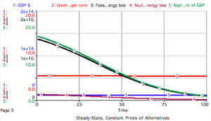
- Steady-State, Constant Prices of Alternatives: The rates of growth of GDP, population and labour force are set to zero to give a steady-state. The rate of growth of labour productivity is maintained at the same level as in the BAU scenario. The average annual hours worked per employed worker declines at almost the same rate as productivity increases so that the rate of unemployment remains virtually unchanged. (Such a decline in time spent at work begins to capture an important aspect of development as defined by Professor Daly, i.e. a qualitative, beneficial change in peoples’ lives.) The same assumptions are made about energy prices as in the BAU scenario.
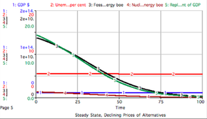
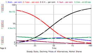
- Steady-State, Declining Prices of Alternatives: This is the same as scenario 2 except that the price of energy from geothermal, hydro, solar thermal, photovoltaic, and wind declines at 0.5% per year to reflect gains from technological improvements and economies of scale as market share increases. The price of biomass is kept constant since as its scale increases it will encounter increased competition from other land uses that may, in fact, make energy from biomass more rather than less expensive over time.
These assumptions are summarized in table 1 and results from the six scenarios are shown in figures 2 - 7.
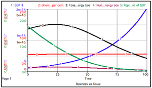


The BAU scenario shown in figures 2 and 3 is not presented as a realistic possibility for the future of the U.S.A. over the next 100 years. It is implausible that [population] of the U.S.A. will more than triple to 928 million but that is what would happen if it continues to increase at a rate of 1.2% per year which was the average annual rate of growth in population from 1990 to 2000. Equally implausible because of the adverse implications for resource use and environmental degradation, is a nineteen-fold increase in real GDP and yet this would be the outcome of a 3% annual growth rate for 100 years. It is the implausibility of projected levels of growth such as these that underlie much of the interest in and case for a [economy]. The BAU scenario scopes out implications of the continuation of past trends. It does not represent a likely or desirable future.
In the BAU scenario total energy use increases three-fold. Energy from fossil fuels and nuclear rise for about 20 years even though their market shares decline throughout the 100 year simulation as they become increasingly more costly relative to the renewable alternatives. The replacement cost of non-renewable energy as a per cent of GDP declines from 14.3 to 0.2 at the end of 100 years in this scenario since GDP is so large and the market share of fossil fuels and nuclear falls to very low levels.
The second scenario shown in figures 4 and 5 illustrates a steady-state: GDP and population are constant. Total energy use declines in response to an increase in the weighted price of energy. After about 80 years total energy use virtually stabilizes because the market shares of the now relatively cheaper renewable energy sources with unchanging prices, have such a large market share that the weighted price of energy also stabilizes and GDP is stable as well. The market shares of the four energy sources is the same as in the BAU scenario because market shares depend only on prices which are the same in both scenarios. Throughout this scenario, the replacement cost of non-renewable energy declines in parallel with the decline in the use of fossil fuels and nuclear energy.
The only difference between the second and third scenario is that in this steady-state scenario the price of the composite renewable energy source (geothermal, hydro, solar thermal, photovoltaic, and wind) declines at 0.5% a year rather than stays constant while the price of biomass remains constant. Over the 100 year simulation period both sources of renewable energy become increasingly competitive with non-renewable energy sources but biomass less so than the composite alternative. The main difference that this makes is with respect to market shares as shown by comparing figures 5 and 7. In figure 7 the composite renewable energy source ends up with 91% of the energy market and biomass with 8% whereas in figure 5 after 100 years their shares are about equal at 45% each.
These scenarios suggest that energy prices can be very important in determining the role that non-renewable and renewable sources of energy have played and will play in determining their use. Energy prices have never simply been set by the market without considerable government intervention through a vast array of subsidies, taxes, direct investment, purchases and regulation. Much of the impact of these interventions has been on prices, directly via gasoline taxes for example, and indirectly through measures such as more or less stringent regulatory limits. The same will be true in the future so while we can get an insight into the potential impact of prices on the replacement of non-renewable energy with renewable energy, it will be as much a matter of public policy and inter-national politics as geology, biology and engineering as to what these prices will be.
Equally telling are the very different implications of continuous growth in GDP and population versus a steady-state. These are placed in stark contrast in the simulations described above. Of course, it is most unlikely that the economy of the USA would suddenly switch to a steady-state defined either in terms used in the model (stable GDP and population) or using a purely physical definition as proposed by Professor Daly. What is more realistic is that it will converge to a steady-state over a period of decades, in a more or less smooth process of transition. This steady-state model gives little insight into what such a process of convergence might look like and how other matters of concern such as the alleviation of poverty, the governments fiscal position, employment levels and greenhouse gas emissions might simultaneously be addressed in a transition to a steady-state. For this we turn to the second simulation model, LowGrow, which was developed to examine considerations such as these for the Canadian economy based on low and no growth.
Managing without Growth[2]
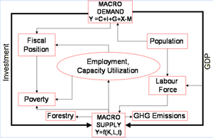
LowGrow is an interactive computerized model of the Canadian economy designed to explore different assumptions, objectives and policy measures related to slowing the rate of economic growth. Figure 8 shows the simplified structure of LowGrow. At the top, aggregate demand (GDP) is determined in the conventional way as the sum of consumption expenditure (C), investment expenditure (I), government expenditure (G), and the difference between exports (X) and imports (I.) There are separate equations for each of these components in the model, estimated with Canadian data from 1981 to 2005. Production in the economy is estimated by a Cobb-Douglas production function in which output (GDP) is a function of employed labour (L) and employed capital (K). The time variable (t) represents changes in productivity from improvements in technology, labour skills and organization. The production function is shown at the bottom of Figure 8. It estimates the labour (L) and employed capital (K) required to produce the GDP (aggregate demand) allowing for changes in productivity over time.[3]
There is a second important link between aggregate demand and the production function shown in figure 8 by the arrow connecting aggregate demand and the production function. Investment expenditures (net of depreciation) which are part of aggregate demand, add to the stock of capital in the economy. Also over time, capital and labour become more productive. It follows that without an increase in GDP these increases in capital and productivity reduce the requirements for labour. Unless an alternative approach is adopted, growth in GDP is needed to prevent unemployment increasing as the productive capacity of the economy expands.
LowGrow includes population growth, which is exogenous, and growth in the labour force, which is estimated as a function of GDP and population. Population is also one of the variables that determines the consumption expenditures in the economy.
There is no monetary sector in LowGrow. For simplicity it is assumed that the Bank of Canada, Canada’s central bank, regulates the money supply to keep inflation at or near the target level of 2 percent per year. LowGrow includes an exogenously set rate of interest. A higher cost of borrowing discourages investment, which reduces aggregate demand. It also raises the cost to government of servicing its debt. LowGrow warns of inflationary pressures when the rate of unemployment falls below 4 percent but the price level is not included as a variable in the model.
While LowGrow lacks these features, it includes others that are particularly relevant for exploring low and no growth scenarios. LowGrow includes emissions of carbon dioxide and other greenhouse gases, a carbon tax, a forestry sub- model, provision for redistributing incomes, and HPI-2, the UN’s Human Poverty Index for selected OECD countries. (United Nations Development Programme, 2006). LowGrow allows additional funds to be spent on health care and on programs to reduce adult illiteracy (both included in HPI-2) and estimates their impacts on longevity and adult literacy with equations obtained from the literature.
Implications of changes in the level of government expenditures can be simulated in LowGrow through a variety of fiscal policies including a balanced budget and an annual percentage change that can vary over time. LowGrow keeps track of the overall fiscal position of all governments combined as measured by the ratio of the combined debt of all levels of government to GDP.
In LowGrow, as in the economy that it represents, economic growth is driven by: net investment which adds to productive assets, growth in the labour force, growth in productivity, growth in the trade balance (i.e. the difference between exports and imports), growth in government expenditures and growth in population. Low and no growth scenarios can be examined by reducing the rates of increase in each and any combination of these factors. In an economy that is dependent on economic growth a sudden dislocation in any and all of these growth drivers can be extremely disruptive as witnessed in the global recession that began in 2008. But as Professor Daly reminds us ‘a failed growth economy and a [economy] are not the same thing; they are the very alternatives we face.’ (Daly, 2008. Also O.Neill, 2008) LowGrow can show how catastrophic a cessation of growth could be if all of the contributors to growth were to fail suddenly and simultaneously. (Victor, 2008, 178-180) The model can also show that a more measured convergence to a steady-state might be achieved if approached systematically over a number of years.
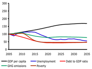
One example of a steady-state scenario for the Canadian economy is shown in figure 9 which displays the time path of five key variables all indexed to a value of 100 in 2005: GDP per capita, the rate of unemployment, greenhouse gas (GHG) emissions, poverty, and the debt to GDP ratio. In this scenario a variety of measures are phased in over a 10 year period stating in 2010. The rate of growth in GDP per capita begins to slow down and falls to zero by around 2030. Since population growth is declining to zero by about the same time, GDP (not shown) also ceases to grow. As figure 9 shows, this decline in the rate of economic growth is accompanied by a reduction in the rate of unemployment to 4% by 2035 (commonly regarded as full-employment in Canada), a substantial reduction in the level of poverty as measured by the UN’s Human Poverty Index, a 25% reduction in greenhouse gas emissions, and a decline then stabilization of the ratio of government debt to GDP.
Each of these outcomes can be traced to one or a few specific changes although they also result from the interactions and feedbacks contained in the structure of LowGrow. The reduction in the growth in GDP per capita results from reduced net investment, a slower rate of increase in the productivity, stabilization of government expenditure, and balanced international trade. Increases in consumption expenditure slow as a result of the lower rate of economic growth brought about by these other changes. A decline in the rate of growth of population coincides with the decline in GDP per capita so that in this steady-state scenario, growth in GDP is also reduced, eventually to zero.
The rate of unemployment is reduced by a 15 per cent reduction in the average number of hours worked by Canadians by 2035, effectively sharing out a stabilized level of labour among a larger number of employees. Even then the average time spent by Canadians would be higher than levels already reached in 2007 in some European countries. (OECD, 2008)
The reduction in poverty shown in figure 9 comes from a lower rate of unemployment and a redistribution of income to bring all Canadians up to the ‘low income cut-off’ (Giles, 2004) and widely used as the unofficial measure of economic poverty in Canada. Poverty is also reduced in this scenario through an expansion of adult literacy programs and health care which address other components of the UN’s Human Poverty Index.
The decline and stabilization of the ratio of government debt to GDP starts from the fiscal regime existing in Canada in 2005, the base year for the simulation. Between 2005 and 2009 this regime changed for several reasons. In particular the federal government reduced the General Sales Tax from 7% to 5%, substantially reducing the federal budget surpluses that this level of government had been running for several years. In late 2008 when the global recession took hold in Canada, revenues for all three levels of government declined and expenditures increased so that the decline in the debt to GDP ratio shown at the start of the scenario in figure 9, before the various measures in the simulation which start in 2010 take effect, did not materialize. This outcome is a reminder that LowGrow is designed to illuminate possibilities for the longer term rather than for simulating short-term changes in the economy.
The reduction in greenhouse gas emissions shown in figure 9 come from a combination of the ongoing decline in greenhouse gas intensity, assumed to continue at the same rate as the rate of increase in overall productivity (which is reduced in this scenario but remains positive), and the introduction of a revenue-neutral carbon tax on energy related GHG emissions. A cap and trade system which resulted in a similar price on these emissions to the carbon tax would have a similar effect.
Beyond 2035 further adjustments would be required to some of the growth drivers to maintain a stable GDP per capita so that the scenario shown in figure 9 is a quasi steady-state. Increases in productivity could continue without increasing GDP if the gains are enjoyed as reduced time spent in paid employment rather than as increased output . Further reductions in greenhouse gas emissions would be stimulated by an increase in the carbon tax.
This brief account of a possible transition to a [economy] answers some questions (i.e. it is feasible to have full employment, much reduced poverty and green house gas emissions, and maintain fiscal balance without relying on economic growth) and raises others. For example, is the top-down, heavy hand of government required or is it just as important, indeed essential, that a steady-state come about in response to changes initiated at the grass roots? Will a [economy] engender more rigid, controlling political and social institutions or will people have more freedom to choose how they spend their time as individuals, families and communities? (They can expect more freedom from the negative environmental impacts of the activities of others.) In a [economy] will it become more difficult to achieve an equitable distribution of income and wealth because the pie is no longer increasing, or easier because other measures of success will have supplanted material living standards? Will paid employment and the private ownership of capital remain the principal means by which income is distributed or will new arrangements be required, and if so, how will they affect incentives to work, save and invest? Is it feasible for a single country to strive for a [economy] if the rest of the world pursues growth as usual? Will it help or hinder developing countries to achieve their development objectives if rich countries pursue a steady-state for their economies? What will a [economy] mean for the rate of profit, the rate of interest, and the monetary system; will it be necessary to limit the outflow of capital as it pursues higher profits elsewhere? What are the resource use and waste generation levels required to sustain the economy at the steady-state level of GDP per capita in 2035 which is projected to be over 50% higher in 2035 than in 2005? Are these levels compatible with the biophysical limits that are a major reason for contemplating a steady-state future? Is this kind of scenario compatible with capitalism? Will new and different types of business and labour organizations be required?
On this last question Robert Solow, one of the architects of the modern theory of economic growth, is reported as saying: ‘There is no reason at all why capitalism could not survive without slow or even [with] no growth.’ (Stoll, 2008) Booth is more circumspect when he says that ‘for a steady-state macroeconomy to function effectively, the requirements at a macroeconomic level are an incomes policy, an expanded government sector, and a reduction in the workweek, and the central need at a microeconomic level may be new organization forms that embody principles of economic democracy…(op.cit . 169)
With respect to the larger rationale for a [economy], Solow showed sympathy for concerns not usually heard from mainstream economists when he observed that ‘it is possible that the US and Europe will find that…either continued growth will be too destructive to the environment and they are too dependent on scarce natural resources, or that they would rather use increasing productivity in the form of leisure.’ (ibid. 94) The case for a steady state economy could not have been stated more succinctly.
Conclusion
It is more than 160 years since John Stuart Mill wrote favourably about the [economy] and over 30 years since Herman Daly wrote the book, so to speak, on the subject. In the mean time economic growth has proceeded apace, and for the past half-century or so has been the over-arching economic policy objective of countries and their governments around the world. With the emergence of ‘sustainable development’ in the 1980s as a possible alternative paradigm, the primacy of economic growth has been called into question and in some circles at least, more attention has begun to be paid to the environmental and social dimensions of development. New measures of progress have been proposed such as the Index of Sustainable Development (Daly and Cobb, 1994, 443-507), the Genuine Progress Index (Redefining Progress, 2007), Genuine Wealth (Hamilton, 2006), and the Human Development Index (United Nations Development Programme, 2006). These take a broader view of progress than just GDP and GDP per capita. Likewise measures such as the Ecological Footprint (Wackernagel, 1996), the Living Planet Index (Hails, 2006), and HANPP (Haberl, 2007) provide quantitative estimates of the environmental burden placed on the planet by people and our economies. The Happy Planet Index offers yet another perspective by measuring a nation’s economic efficiency as the ratio of well-being (based on life satisfaction and life expectancy) to the ecological footprint. (NEF, 2009)
To a greater or lesser extent the rationale for these alternative indicators stem from concerns similar to those expressed by the many contributors to steady-state economics, some of whose ideas have been discussed in this chapter. Yet it would be premature to say that the option of a [economy] has made it on to the public or political agenda in a significant way. The OECD, for example, remains committed to economic growth even as it writes about sustainable development and struggles to reconcile the demands of growing economies with the biophysical limits of the planet. (Strange, 2009). In contrast, the UK’s Sustainable Development Commission has questioned the viability of economic growth over the long term and raised for serious consideration the possibility of seeking prosperity without growth. (Jackson, 2009). Going even further, the governments of Bolivia, Cuba, Dominica, Honduras, Nicaragua and Venezuela declared in 2009 that ‘the global economic, climate change, food and energy crises are products of the decadence of capitalism that threatens to put an end to the existence of life and the planet. To avoid this outcome it is necessary to develop an alternative model to that of the capitalist system.’ (ALBA, 2009)
In developed countries outside officialdom, there is a dialogue especially in France about ‘degrowth’ or décroissance (Latouche, 2007), a lively website discussing steady-state economics run by the Centre for Advancement of the Steady-State Economy in the United States (CASSE, 2009), and numerous energy, environment and other groups increasingly making the links between their more specific concerns and the character and conduct of the economy.
In the words of Herman Daly ‘The closer the economy approaches the scale of the whole Earth the more it will have to conform to the physical behaviour mode of the Earth. That behaviour mode is a steady-state – a system that permits qualitative development but not aggregate quantitative growth.’ (Daly, 2008, 1) Whether we will make a careful and thoughtful transition to the steady-state remains to be seen but at least through the work of Professor Daly and all those he has inspired, we are better able to delineate the options.
Cited Literature
- ALBA. 2009. Document of the Bolivarian Alternative for the Peoples of Our Americas (ALBA) countries for the Fifth Summit of the AmericasCumaná.
- Booth D. E. 1998. The Environmental Consequences of Growth: Steady-State Economics as an Alternative to Ecological Decline. Routledge. London; New York.
- Boulding K. E. 1966. Economics of the Coming Spaceship Earth. In Environmental Quality in a Growing Economy: Essays from the Sixth RFF Forum. Jarrett H., Ed.: 3-14. Johns Hopkins Press. Baltimore.
- Boulding K. E. 1973. The Shadow of the Stationary State. In The no-Growth Society. Olson M. and H. H. Landsberg, Eds.: 89-101. W.W. Norton & Company. New York.
- Burkett P. 2004. Marx's reproduction schemes and the environment. Ecological Economics. 49: 457-467.
- CASSE. 2009. Center for the Advancement of the Steady-State Economy. 20 April 2009.
- Daly H. E. 1968. On Economics as a Life Science. Journal of Political Economy. 76: 392.
- Daly H. E. 1977. Steady-State Economics: The Economics of Biophysical Equilibrium and Moral Growth. W. H. Freeman. San Francisco.
- Daly H. E. 2008. A Steady-State Economy.
- Daly H. E., J. B. Cobb & C. W. Cobb. 1994. For the Common Good: Redirecting the Economy Toward Community, the Environment, and a Sustainable Future. Beacon Press. Boston.
- Daly H. E. & J. C. Farley. 2004. Ecological Economics: Principles and Applications. Island Press. Washington DC.
- Gately D. & H. G. Huntington. 2002. The Asymmetric Effects of Changes in Price and Income on Energy and Oil Demand Oil Price and Policy. 23: 19-56.
- Georgescu-Roegen N. 1971. The Entropy Law and the Economic Process. Harvard University Press. Cambridge, Mass.
- Georgescu-Roegen N. 1980. Selections from "Energy and Economic Myths". In Economics, Ecology, Ethics. Essays Toward a Steady-State Economy. Daly H. E., Ed.: 61-81. W.H. Freeman and Company. San Francisco.
- Giles P. 2004. Low Income Measurement in Canada. 75F0002MIE - 011: 20.
- Haberl H., K. Erb & F. Krausmann. 2007. Human appropriation of net primary production (HANPP). In Internet Encyclopedia of Ecological Economics. Neumeyer E., Ed.International Society for Ecological Economics.
- Hails C., J. Loh & S. Goldfinger. 2006. Living Planet Report 2006.
- Hamilton K. 2006. Where is the wealth of nations? Measuring capital for the 21st century.
- Hubber M.K. 1956. Nuclear Energy and the Fossil Fuels, Publication no. 95, Shell Development Corporation, Houston.
- Hubbert M. K. 1974. M. King Hubbert on the Nature of Growth.
- Jackson T. 2009. Prosperity without Growth? .
- Keynes J. M. 1935. The General Theory of Employment Interest and Money. Harcourt-Brace. New York.
- Keynes J. M. 1963. Essays in Persuasion. W.W. Norton & Company. New York.
- Latouche S. 2007. De-growth: an electoral stake? International Journal of Inclusive Democracy. 3.
- Meadows, D.H. et al. 1972. The Limits to Growth. Earth Island Press, London
- Mill J. S. 1970. Principles of political economy: with some of their applications to social philosophy.
- NEF, 2009. The Unhappy Planet Index 2.0.
- OECD. 2008. Average annual hours actually worked per worker Vol 2008 release 01.
- Redefining Progress. 2007. Genuine Progress Indicator.
- Rivers N. and M. Jaccard 2005. “Combining Top-Down and bottom:Up Approaches to Energy-Economy Modeling Using Discrete Choice Methods”, The Energy Journal, 26, 1 83 - 106
- Soddy F. 1926. Wealth, Virtual Wealth and Debt: The Solution of the Economic Paradox. Allen & Unwin. London.
- Stoll S. 2008. Fear of Fallowing. The spectre of a no-growth world. Harper's Magazine. 88-94.
- Strange T., & A. Bayley. 2009. Sustainable Development. Linking Economy, Society, Environment. OECD. Paris.
- Turner, G.M. 2008. “A comparison of The Limits to Growth with 30 years of reality". Global Environmental Change. 18, 3, 397-411
- United Nations Development Programme. 2006. Human Development Report 2006.
- US Energy Information Administration. 2008. Renewable Energy Trends in Consumption and Electricity 2006 Edition.
- Victor P. A. 2009. Ecological Economics and Economic Growth. The Year in Ecological Economics (forthcoming). 1.
- Wackernagel M. & W. E. Rees. 1996. Our Ecological Footprint: Reducing Human Impact on the Earth. New Society Publishers. Gabriola Island, Canada and Philadelphia, US.
Notes
This is a chapter from Herman Daly Festschrift (e-book). Previous: Chapter 21|Table of Contents (Herman Daly Festschrift: Herman Daly and the Steady State Economy) |Next: Chapter 23 (Herman Daly Festschrift: Herman Daly and the Steady State Economy)
Citation
Victor, P. (2013). Herman Daly Festschrift: Herman Daly and the Steady State Economy. Retrieved from http://editors.eol.org/eoearth/wiki/Herman_Daly_Festschrift:_Herman_Daly_and_the_Steady_State_Economy- ↑ See also Victor (1979)
- ↑ This section of the paper is adapted from chapter 10 of Victor (2008) where more details of LowGrow and more scenarios can be found. Chapter 11 provides a discussion of policies for managing without growth.
- ↑ The Cobb-Douglas production function does not represent the throughput and substitution possibilities of the economy between manufactured and natural capital. Its role in LowGrow is only to estimate the relation between inputs of labour and capital required to generate GDP.