Excel 2010

PivotCharts

PivotCharts are like regular charts, except they display data from a PivotTable. As with a regular chart, you'll be able to select a chart type, layout, and style to best represent the data. In this example, we'll use a PivotChart so we can visualize the trends in each sales region.

To create a PivotChart:

1. Select any cell in your PivotTable. The Options tab will appear on the Ribbon.
2. From the Options tab, click the PivotChart command.
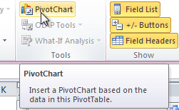   The PivotChart command
3. From the dialog box, select the desired chart type (3-D Clustered Column, for example), then click OK.
   Selecting a chart type
4. The PivotChart will appear in the worksheet. If you want, you can move it by clicking and dragging.
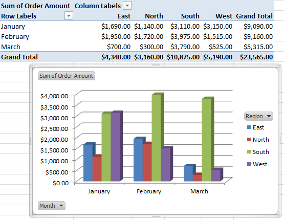   A PivotChart

If you make any changes to the PivotTable, the PivotChart will adjust automatically.