Excel 2010

To create a PivotTable:

1. Select the table or cells (including column headers) containing the data you want to use.
2. From the Insert tab, click the PivotTable command.
   The PivotTable command
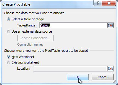
3. The Create PivotTable dialog box will appear. Make sure the settings are correct, then click OK.
   The Create PivotTable dialog box
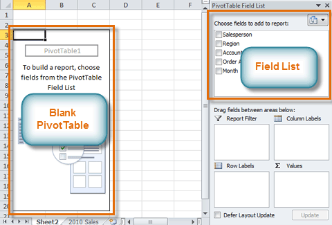
4. A blank PivotTable will appear on the left, and the Field List will appear on the right.
   The Blank PivotTable and Field List

To add fields to the PivotTable:

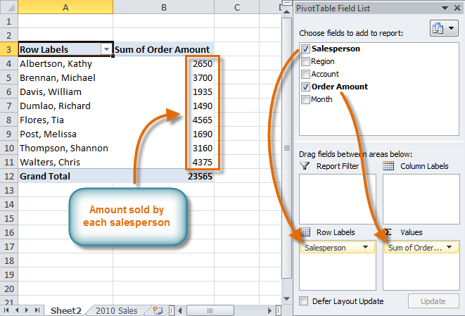
Now, you'll need to decide which fields to add to the PivotTable. Each field is simply a column header from the source data. It may be helpful to recall the question you are trying to answer. In this example, we want to know the total amount sold by each salesperson, so we'll just need the Order Amount and Salesperson fields.

1. In the Field List, place a checkmark next to each field you want to add.
2. The selected fields will be added to one of the four Areas below the Field List. In this example, the Salesperson field is added to the Row Labels area, and the Order Amount is added to the Values area. If a field is not in the desired area, you can drag it to a different one.
3. The PivotTable now shows the amount sold by each salesperson.
   Adding fields to the PivotTable

Just like with normal spreadsheet data, you can sort the data in a PivotTable using the Sort & Filter command in the Home tab. You can also apply any type of formatting you want. For example, you may want to change the Number Format to Currency. However, be aware that some types of formatting may disappear when you modify the PivotTable.

If you change any of the data in your source worksheet, the PivotTable will not update automatically. To manually update it, select the PivotTable and then go to OptionsRefresh.