Excel 2010

Pivoting data

One of the best things about PivotTables is that they let you "pivot" the data in order to look at it in a different way. This allows you to answer multiple questions and even experiment with the data to learn new things about it.

In our example, we used the PivotTable to answer the question, "What is the total amount sold by each salesperson?" But now we'd like to answer a new question, such as "What is the total amount sold in each month?" We can do this by simply changing the Row Labels.

To change the Row Labels:

1. Drag any existing fields out of the Row Labels area, and they will disappear.
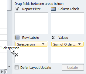   Dragging a field out of Row Labels
2. Drag a new field from the Field List into the Row Labels area. In this example, we're using the Month field.
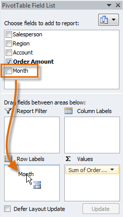   Dragging a new field into Row Labels
3. The PivotTable will adjust to show the new data. In this example, it now shows us the total Order Amount for each month.
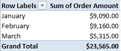   The updated PivotTable

To add Column Labels:

So far, our PivotTable has only shown one column of data at a time. In order to show multiple columns, we'll need to add Column Labels.

1. Drag a field from the Field List into the Column Labels area. In this example, we're using the Region field.
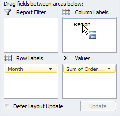   Adding a field to Column Labels
2. The PivotTable will now have multiple columns. In this example, there is a column for each region.
   The updated PivotTable