Google Sheets
Sorting and Filtering Data
To create a filter:
In our example, we will apply a filter to narrow down the data in our spreadsheet. We will display only the animal and nature books.
- Click any cell that contains data.
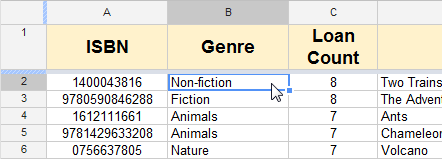 Selecting a cell
 - Click the Filter button.
 The Filter button
 - A drop-down arrow
 appears in each column header.
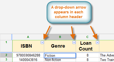 Drop-down arrows in the column headers
 - Decide which column you will apply a filter to. Click the column's drop-down arrow, and a filtering options box appears. You will see the values from that column as a checklist inside the box. In our example, the checklist is showing all of the genres we typed in the column.
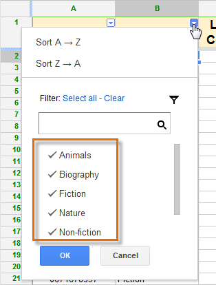 The checklist of column values
 - Click Clear to remove all of the checks.
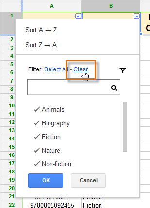 Clicking Clear
 - Select the data you wish to display on the spreadsheet. In this example, we will select Animals and Nature. Click OK.
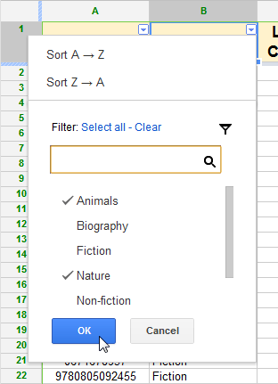 Setting the filter
 - The sheet will be filtered according to your data selection. A filter symbol
 appears in the filtered column's header cell.
 Viewing the filtered results
Applying multiple filters
When you create a filter in your spreadsheet, each column header on your sheet will have a drop-down arrow for creating new filters. Filters are cumulative, meaning you are free to use as many as you need to narrow your data to the desired result. In the image below, the library's books on loan list has been filtered by genre and loan count. As a result of the two filters, Google Spreadsheets displays animal and nature books that have been loaned more than four times.
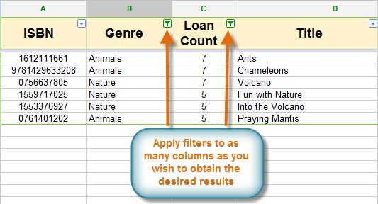 Viewing multiple filters
To clear all filters:
- Click the Filter button, and the spreadsheet will return to its original appearance.
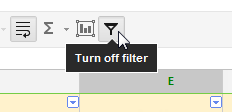 Removing a filter


