Google Sheets

Introduction

Google Spreadsheets allows you to analyze and work with a significant amount of data. As you add more content to your spreadsheet, knowing how to locate specific information in it becomes important. Spreadsheets allows you reorganize your data by sorting and applying filters to it. You can sort your data by arranging it alphabetically or numerically, or you can apply a filter to narrow down the data and hide some of it from view.

In this lesson, you will learn how to sort data to better view and organize the contents of your spreadsheet. You will also learn how to filter data to display only the information you need.

Sorting and filtering data

When working with Google Spreadsheets, sometimes you may wish to reorganize the data so you can easily find the information you're looking for. Sorting allows you to change or customize the order of your spreadsheet data. For example, in preparation for a charity event you could organize the volunteer list by name and T-shirt size so you can determine how many T-shirts you need in each size.

Filters can be applied in many different ways to improve the performance of your worksheet. They are useful for displaying only the data that interests you. For example, you could apply a filter to a party guest list to view only the people who responded to the invitation, or sort the genres of a song list to display only rock and roll songs or classical music.

Types of sorting

When sorting data, it's important to first decide if you would like the sort to apply to the entire sheet or to a selection of cells. 

• Sort sheet organizes all of the data in your spreadsheet by one column. Related information across each row is kept together when the sort is applied. In the image below, the Name column has been sorted to display the client names in alphabetical order. Each client's address information has been kept with each corresponding name.
  
  An alphabetically sorted sheet
  
• Sort range sorts the data in a range of cells. When working with a sheet that contains several tables, you may wish to sort the data of a single table. Sorting a range will not affect the data on the rest of the sheet, and it will keep related information across the row together.
  
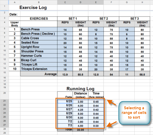  Sorting a range of cells

To sort a sheet:

In our example, we will sort a library's books on loan list to easily see which books have been checked out most often. We will freeze the header row so the header labels will not be included in the sort.

1. Click View and hover the mouse over Freeze rows. Select Freeze 1 row from the menu that appears.
   
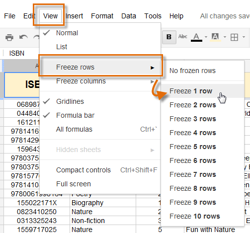   Freezing the header row
2. The header row freezes. Decide which column will be sorted, then click on a cell in the column. In our example, we will click on a cell in the Loan Count column to reorganize the books by the number of times they have been loaned.
   
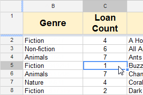   Selecting a cell in the desired column
3. Click Data and select Sort Sheet by column, A-Z (ascending) or Sort Sheet by column, Z-A (descending). In our example, we will select Sort Sheet by column, Z-A to display the most often loaned books at the top of the list.
   
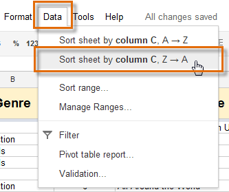   Selecting Sort sheet by column
4. The sheet will be sorted according to your selection.
   
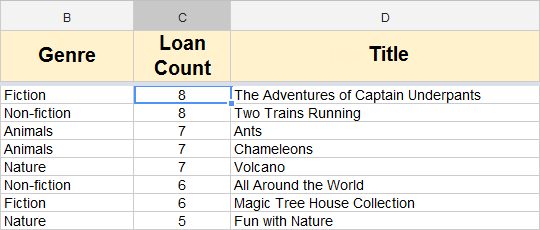   The sorted data

To sort a range:

In our example, we will sort a range of data in an exercise log. We will reorganize the data to display the jogging distance in ascending order.

1. Highlight the range of cells you wish to sort. In this example, we will select the range C21:E27.
   
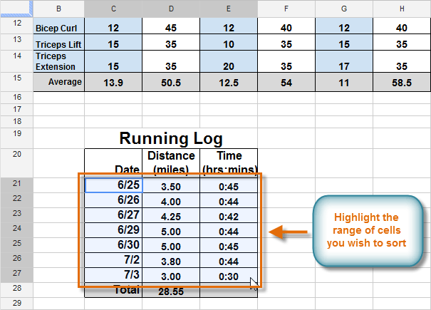   Highlighting a range of cells
2. Click Data and select Sort range... from the drop-down menu.
   
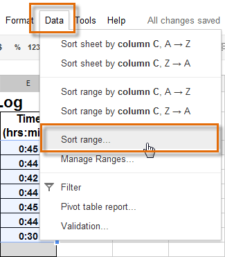   Selecting Sort range...
3. The Sorting dialog box appears. Select the desired column you wish to sort by, then select ascending or descending.
4. Click Sort.
   
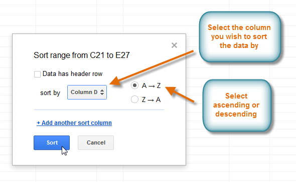   Setting the sort range options
5. The range will be sorted according to your selections (in our example, the data has been sorted in ascending order according to the distance column).
   
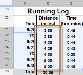   The sorted range of cells

To create a filter:

In our example, we will apply a filter to narrow down the data in our spreadsheet. We will display only the animal and nature books.

1. Click any cell that contains data.
   
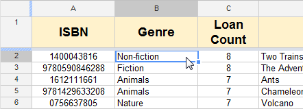   Selecting a cell
2. Click the Filter button.
   
   The Filter button
3. A drop-down arrow appears in each column header.
   
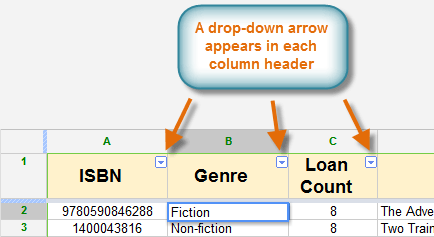   Drop-down arrows in the column headers
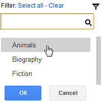
4. Decide which column you will apply a filter to. Click the column's drop-down arrow, and a filtering options box appears. You will see the values from that column as a checklist inside the box. In our example, the checklist is showing all of the genres we typed in the column.
   
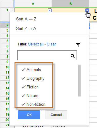   The checklist of column values
   
5. Click Clear to remove all of the checks.
   
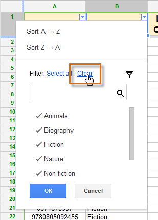   Clicking Clear
6. Select the data you wish to display on the spreadsheet. In this example, we will select Animals and Nature. Click OK.
   
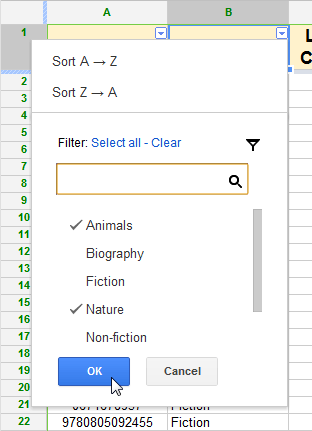   Setting the filter
   
7. The sheet will be filtered according to your data selection. A filter symbol appears in the filtered column's header cell.
   
   Viewing the filtered results

Applying multiple filters

When you create a filter in your spreadsheet, each column header on your sheet will have a drop-down arrow for creating new filters. Filters are cumulative, meaning you are free to use as many as you need to narrow your data to the desired result. In the image below, the library's books on loan list has been filtered by genre and loan count. As a result of the two filters, Google Spreadsheets displays animal and nature books that have been loaned more than four times.

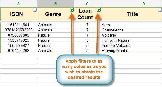Viewing multiple filters

To clear all filters:

• Click the Filter button, and the spreadsheet will return to its original appearance.
  
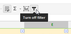  Removing a filter

Challenge!

To work through the challenge, open GCFLearnFree L16: Library Books on Loan and Workout Log and copy the file to your Google Drive. View the instructions below the challenge if you are not sure how to make a copy of the file.

1. Using the Books on Loan sheet, sort the sheet so the books are alphabetized by title.
2. Filter the Due Date column to display only the books that are due on July 14, 2012 (7/14/2012).
3. Try applying a second filter to the sheet.
4. Using the Workout Log sheet, sort the range of cells L21:N27 to display the stationary bike Distance column in descending order.

To copy the example file to your Google Drive:

In these tutorials, we will provide example files you can use to practice what you've learned in each lesson. Because these files are Google Docs we have chosen to share, you will need to copy the file to your Google Drive before you can edit the file.

1. Click the link at the top of this page to open the example file.
2. The example file will appear in a new browser tab or window. If you are not currently signed in to your Google account, locate and click Sign in on the top-right corner of the page.
   
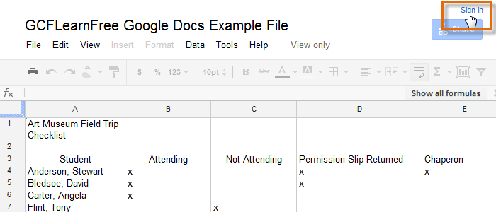   Signing in to your Google Account
3. After you have signed in to your Google account, locate and select File in the toolbar menu and select Make a copy... from the drop-down menu.
   
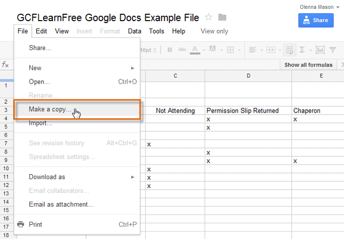   Making a copy of the example file
4. The Copy Document dialog box will appear. Enter a new title for the file, then click OK.
   
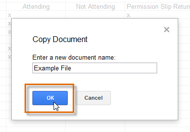   Naming the file and clicking OK
5. The copy of the file will appear in a new browser tab. Now you're ready to start using the example file.
   
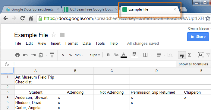   Viewing the copied example file in a new tab