

Excel 2013
PivotTables
PivotCharts
PivotCharts are like regular charts, except that they display data from a PivotTable. Just like regular charts, you'll be able to select a chart type, layout, and style that will best represent the data.
To create a PivotChart:
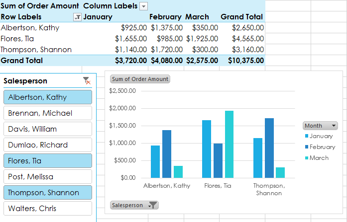
In this example, our PivotTable is showing each person's total sales per month. We'll use a PivotChart so we can see the information more clearly.
- Select any cell in your PivotTable.
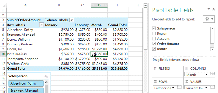 Clicking a cell in the PivotTable
 - From the Insert tab, click the PivotChart command.
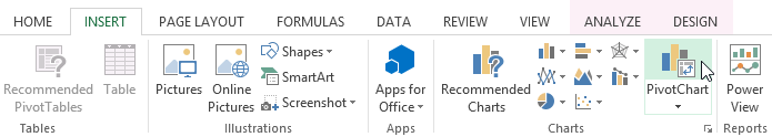 Clicking the PivotChart command
 - The Insert Chart dialog box will appear. Select the desired chart type and layout, then click OK.
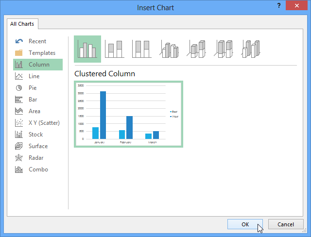 Choosing a chart type and clicking OK
 - The PivotChart will appear.
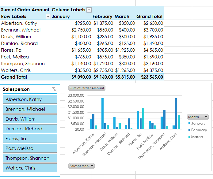 The inserted PivotChart
Try using slicers or filters to change the data that is displayed. The PivotChart will automatically adjust to show the new data.
 Manipulating a PivotChart


