

Excel 2013
PivotTables
Pivoting data
One of the best things about PivotTables is that they can quickly pivot, or reorganize, data, allowing you to look at your worksheet data in different ways. Pivoting data can help you answer different questions and even experiment with the data to discover new trends and patterns.
In our example, we used the PivotTable to answer the question: "What is the total amount sold by each salesperson?" But now we'd like to answer a new question: "What is the total amount sold in each month?" We can do this by simply changing the field in the Rows area.
To change the row:
- Click, hold, and drag any existing fields out of the Rows area. The field will disappear.
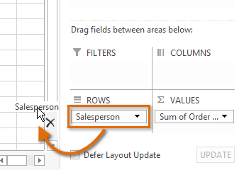 Removing a field
 - Drag a new field from the Field List into the Rows area. In our example, we'll use the Month field.
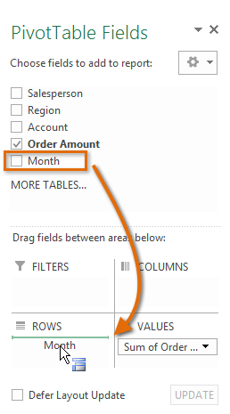 Adding a field
 - The PivotTable will adjust, or pivot, to show the new data. In our example, it now shows the total Order Amount for each month.
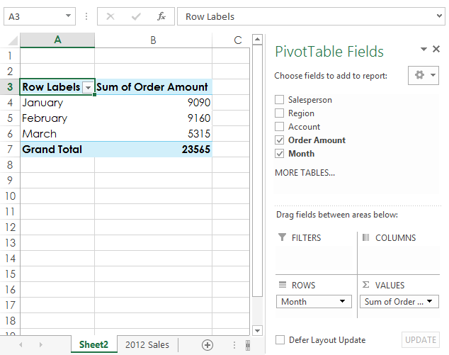 The updated PivotTable
To add columns:
So far, our PivotTable has only shown one column of data at a time. In order to show multiple columns, you'll need to add a field to the Columns area.
- Drag a field from the Field List into the Columns area. In our example, we'll use the Region field.
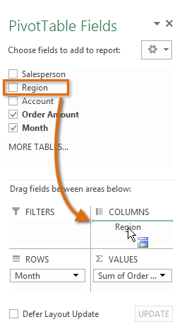 Adding a field to the Column area
 - The PivotTable will include multiple columns. In our example, there is now a column for each region.
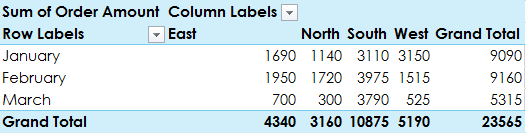 The PivotTable with columns


