Excel 2013

To create a PivotTable:

1. Select the table or cells (including column headers) containing the data you want to use.
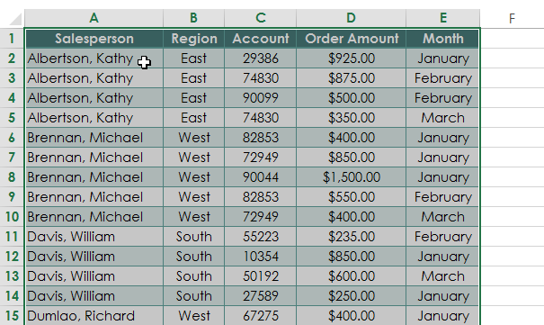   Selecting cells for a PivotTable
2. From the Insert tab, click the PivotTable command.
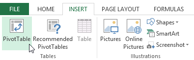   Clicking the PivotTable command
3. The Create PivotTable dialog box will appear. Choose your settings, then click OK. In our example, we'll use Table1 as our source data and place the PivotTable on a new worksheet.
   
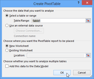   Creating a PivotTable
4. A blank PivotTable and Field List will appear on a new worksheet.
   A blank PivotTable on its own worksheet
5. Once you create a PivotTable, you'll need to decide which fields to add. Each field is simply a column header from the source data. In the PivotTable Field List, check the box for each field you wish to add. In our example, we want to know the total amount sold by each salesperson, so we'll check the Salesperson and Order Amount fields.
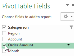   Checking the desired fields
   
6. The selected fields will be added to one of the four areas below the Field List. In our example, the Salesperson field has been added to the Rows area, while the Order Amount has been added to the Values area. Alternatively, you can click, hold, and drag a field to the desired area.
   
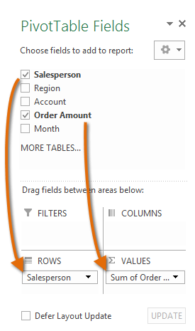   Adding fields to the PivotTable
   
7. The PivotTable will calculate and summarize the selected fields. In our example, the PivotTable shows the amount sold by each salesperson.
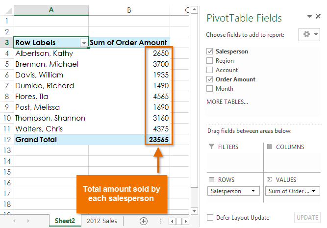   The PivotTable calculating the selecting fields
   

Just like with normal spreadsheet data, you can sort the data in a PivotTable using the Sort & Filter command in the Home tab. You can also apply any type of number formatting you want. For example, you may want to change the Number Format to Currency. However, be aware that some types of formatting may disappear when you modify the PivotTable.

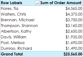A sorted and formatted PivotTable

If you change any of the data in your source worksheet, the PivotTable will not update automatically. To manually update it, select the PivotTable and then go to AnalyzeRefresh.