Excel 2010

Conditional formatting

Video: Conditional Formatting in Excel 2010

Watch the video (3:17).

Conditional formatting applies one or more rules to any cells you want. An example of a rule might be "If the value is greater than 5000, color the cell yellow." By applying this rule to the cells in a worksheet, you'll be able to see at a glance which cells are over 5000. There are also rules that can mark the top 10 items, all cells that are below the average, cells that are within a certain date range, and many more.

To create a conditional formatting rule:

1. Select the cells you want to add formatting to.
2. In the Home tab, click the Conditional Formatting command. A drop-down menu will appear.
3. Select Highlight Cells Rules or Top/Bottom Rules. We will choose Highlight Cells Rules for this example. A menu will appear with several rules.
4. Select the desired rule (Greater Than, for example).
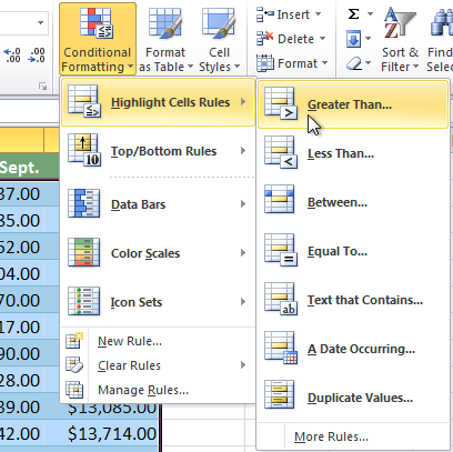   Selecting the Greater Than rule
5. From the dialog box, enter a value in the space provided, if applicable. In this example, we want to format cells that are greater than $5000, so we'll enter 5000 as our value. If you want, you can enter a cell reference instead of a number.
6. Select a formatting style from the drop-down menu.
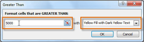   Entering a value and formatting style
7. The formatting will be applied to the selected cells.
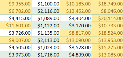   The formatted cells

If you want, you can apply more than one rule to your cells.