Excel 2013

Introduction

Video: Freezing Panes and View Options

Watch the video (4:28).

Whenever you're working with a lot of data, it can be difficult to compare information in your workbook. Fortunately, Excel includes several tools that make it easier to view content from different parts of your workbook at the same time, such as the ability to freeze panes and split your worksheet.

Optional: Download our Lesson 17 Practice Workbook.

To freeze rows:

You may want to see certain rows or columns all the time in your worksheet, especially header cells. By freezing rows or columns in place, you'll be able to scroll through your content while continuing to view the frozen cells.

1. Select the row below the row(s) you wish to freeze. In our example, we want to freeze rows 1 and 2, so we'll select row 3.
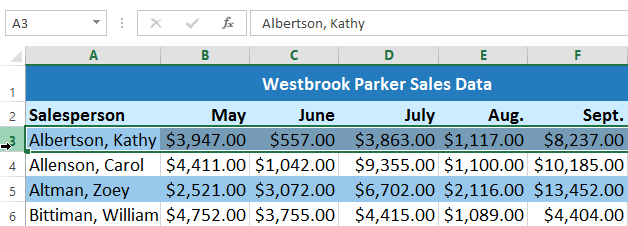   Selecting row 3
2. Click the View tab on the Ribbon.
3. Select the Freeze Panes command, then choose Freeze Panes from the drop-down menu.
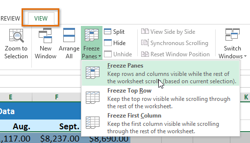   Clicking Freeze Panes
4. The rows will be frozen in place, as indicated by the gray line. You can scroll down the worksheet while continuing to view the frozen rows at the top. In our example, we've scrolled down to row 18.
   
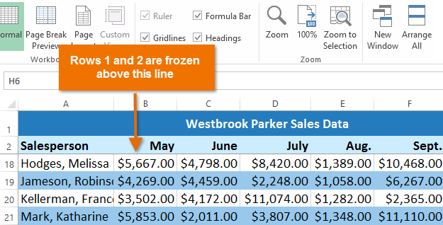   The frozen rows

To freeze columns:

1. Select the column to the right of the column(s) you wish to freeze. In our example, we want to freeze column A, so we'll select column B.
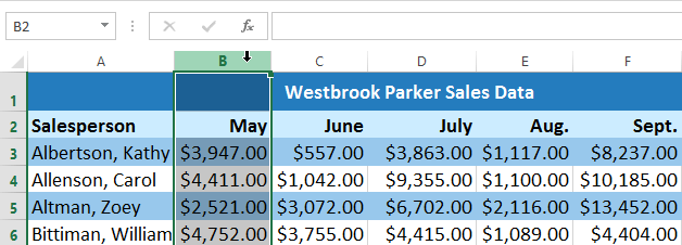   Selecting column B
2. Click the View tab on the Ribbon.
3. Select the Freeze Panes command, then choose Freeze Panes from the drop-down menu.
   Clicking Freeze Panes
4. The column will be frozen in place, as indicated by the gray line. You can scroll across the worksheet while continuing to view the frozen column on the left. In our example, we've scrolled across to column E.
   
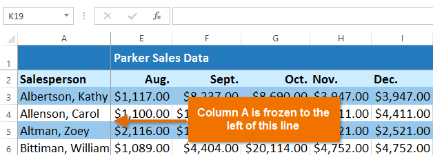   The frozen column

To unfreeze rows or columns, click the Freeze Panes command, then select Unfreeze Panes from the drop-down menu.

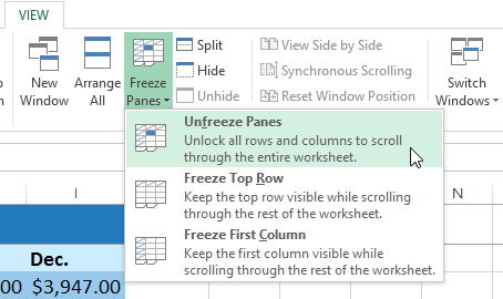Unfreezing a row

If you only need to freeze the top row (row 1) or first column (column A) in the worksheet, you can simply select Freeze Top Row or Freeze First Column from the drop-down menu.

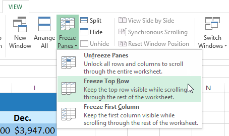Freezing only the top row of a workbook