Excel 2013

Introduction

Video: Conditional Formatting

Watch the video (3:54).

Let's imagine you have a worksheet with thousands of rows of data. It would be extremely difficult to see patterns and trends just from examining the raw information. Similar to charts and sparklines, conditional formatting provides another way to visualize data and make worksheets easier to understand.

Optional: Download our Lesson 26 Practice Workbook.

Understanding conditional formatting

Conditional formatting allows you to automatically apply formatting—such as colors, icons, and data bars—to one or more cells based on the cell value. To do this, you'll need to create a conditional formatting rule. For example, a conditional formatting rule might be: "If the value is less than $2000, color the cell red." By applying this rule, you'd be able to quickly see which cells contain values under $2000.

Conditional formatting marking values less than $2000

To create a conditional formatting rule:

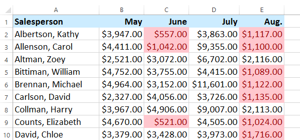
In our example, we have a worksheet containing sales data, and we'd like to see which salespeople are meeting their monthly sales goals. The sales goal is $4000 per month, so we'll create a conditional formatting rule for any cells containing a value higher than 4000.

1. Select the desired cells for the conditional formatting rule.Selecting the desired cells
2. From the Home tab, click the Conditional Formatting command. A drop-down menu will appear.
3. Hover the mouse over the desired conditional formatting type, then select the desired rule from the menu that appears. In our example, we want to highlight cells that are greater than $4000.
   
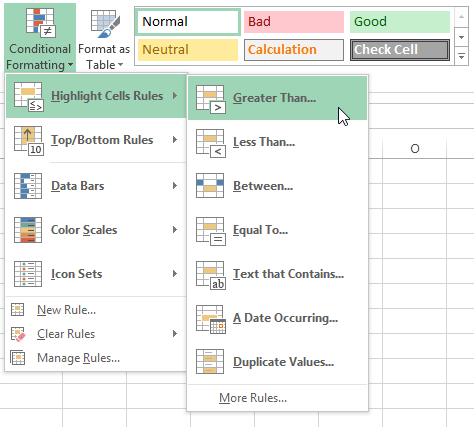   Selecting a conditional formatting rule
4. A dialog box will appear. Enter the desired value(s) into the blank field. In our example, we'll enter 4000 as our value.
5. Select a formatting style from the drop-down menu. In our example, we'll choose Green Fill with Dark Green Text, then click OK.
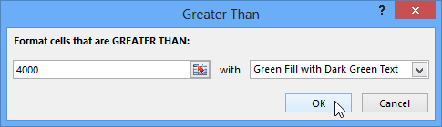   Creating a conditional formatting rule
6. The conditional formatting will be applied to the selected cells. In our example, it's easy to see which salespeople reached the $4000 sales goal for each month.
   
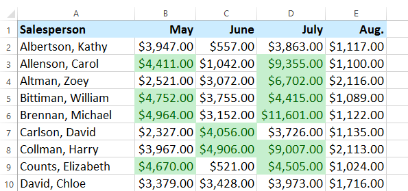   Conditional formatting applied to the data

You can apply multiple conditional formatting rules to a cell range or worksheet, allowing you to visualize different trends and patterns in your data.

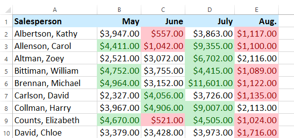A worksheet with multiple conditional formatting rules

To remove conditional formatting:

1. Click the Conditional Formatting command. A drop-down menu will appear.
2. Hover the mouse over Clear Rules, and choose which rules you wish to clear. In our example, we'll select Clear Rules from Entire Sheet to remove all conditional formatting from the worksheet.
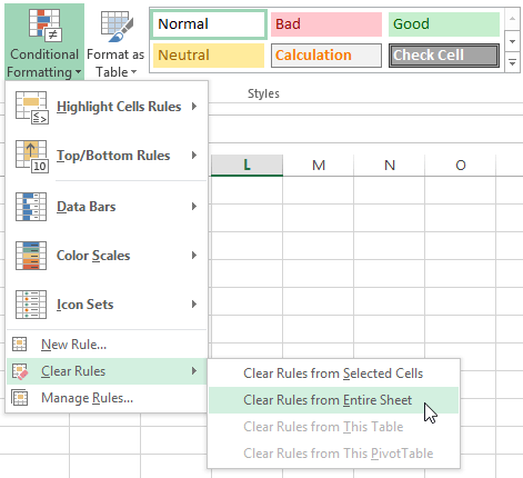   Removing conditional formatting rules
3. The conditional formatting will be removed.
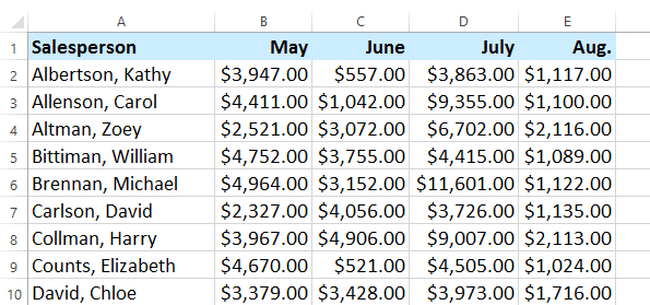   The conditional formatting removed from the worksheet

Click Manage Rules to edit or delete individual rules. This is especially useful if you have applied multiple rules to a worksheet.

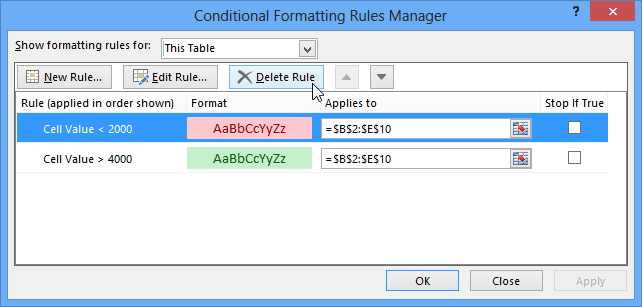Deleting an individual rule