Excel 2013

Introduction

Video: Formatting Cells

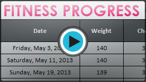Watch the video (4:10).

All cell content uses the same formatting by default, which can make it difficult to read a workbook with a lot of information. Basic formatting can customize the look and feel of your workbook, allowing you to draw attention to specific sections and making your content easier to view and understand. You can also apply number formatting to tell Excel exactly what type of data you’re using in the workbook, such as percentages (%), currency ($), and so on.

Optional: Download our Lesson 9 Practice Workbook.

To change the font:

By default, the font of each new workbook is set to Calibri. However, Excel provides a variety of other fonts you can use to customize your cell text. In the example below, we'll format our title cell to help distinguish it from the rest of the worksheet.

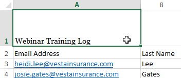
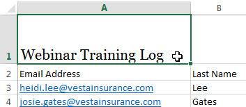
1. Select the cell(s) you wish to modify.
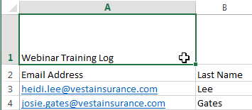   Selecting a cell
2. Click the drop-down arrow next to the Font command on the Home tab. The Font drop-down menu will appear.
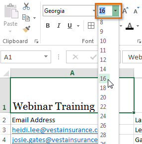
3. Select the desired font. A live preview of the new font will appear as you hover the mouse over different options. In our example, we'll choose Georgia.
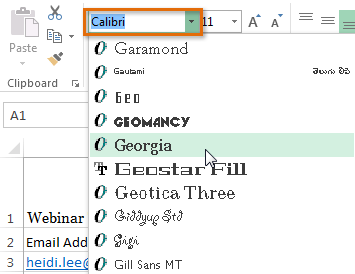   Choosing a font
   
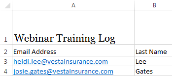
4. The text will change to the selected font .
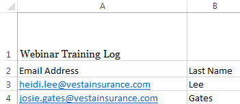   The new font

When creating a workbook in the workplace, you'll want to select a font that is easy to read. Along with Calibri, standard reading fonts include Cambria, Times New Roman, and Arial.

To change the font size:

1. Select the cell(s) you wish to modify.
   Selecting a cell
2. Click the drop-down arrow next to the Font Size command on the Home tab. The Font Size drop-down menu will appear.
3. Select the desired font size. A live preview of the new font size will appear as you hover the mouse over different options. In our example, we will choose 16 to make the text larger.
   Choosing a new font size
4. The text will change to the selected font size.
   The new font size

You can also use the Increase Font Size and Decrease Font Size commands or enter a custom font size using your keyboard.

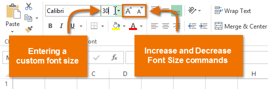Modifying the font size

To change the font color:

1. Select the cell(s) you wish to modify.
   
   Selecting a cell
2. Click the drop-down arrow next to the Font Color command on the Home tab. The Color menu will appear.
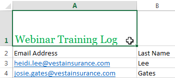
3. Select the desired font color. A live preview of the new font color will appear as you hover the mouse over different options. In our example, we'll choose Green.
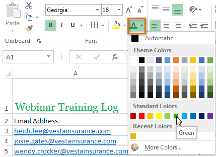   Choosing a font color
4. The text will change to the selected font color.
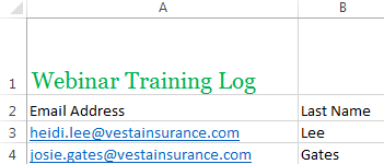   The new font color

Select More Colors at the bottom of the menu to access additional color options.

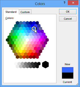Selecting more colors

To use the Bold, Italic, and Underline commands:

1. Select the cell(s) you wish to modify.
   Selecting a cell
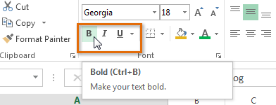
2. Click the Bold (B), Italic (I), or Underline (U) command on the Home tab. In our example, we'll make the selected cells bold.
   Clicking the Bold command
3. The selected style will be applied to the text.
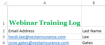   The bold text

You can also press Ctrl+B on your keyboard to make selected text bold, Ctrl+I to apply italics, and Ctrl+U to apply an underline.

Text alignment

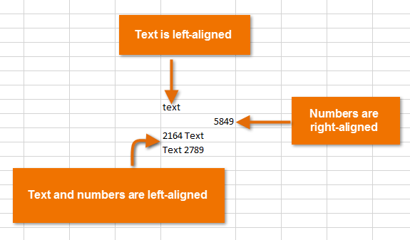
By default, any text entered into your worksheet will be aligned to the bottom-left of a cell. Any numbers will be aligned to the bottom-right of a cell. Changing the alignment of your cell content allows you to choose how the content is displayed in any cell, which can make your cell content easier to read.

Click the arrows in the slideshow below to learn more about the different text alignment options.

• 

  Left align: Aligns content to the left border of the cell

• 

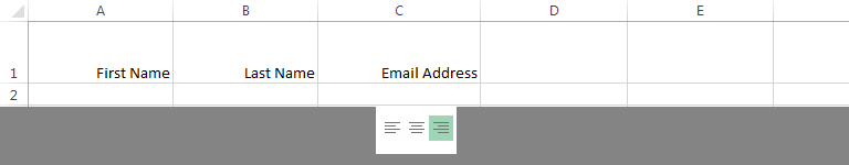
  Center align: Aligns content an equal distance from the left and right borders of the cell

• 

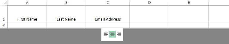
  Right Align: Aligns content to the right border of the cell

• 

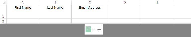
  Top Align: Aligns content to the top border of the cell

• 

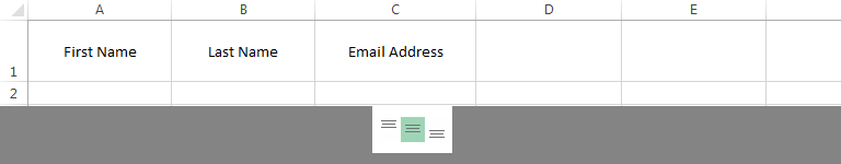
  Middle Align: Aligns content an equal distance from the top and bottom borders of the cell

• 

  Bottom Align: Aligns content to the bottom border of the cell

To change horizontal text alignment:

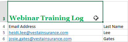
In our examples below, we'll modify the alignment of our title cell to create a more polished look and further distinguish it from the rest of the worksheet.

1. Select the cell(s) you wish to modify.
   Selecting a cell
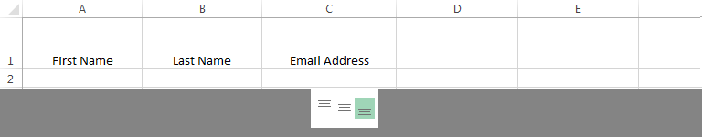
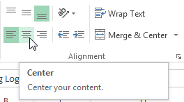
2. Select one of the three horizontal alignment commands on the Home tab. In our example, we'll choose Center Align.
   
   Choosing Center Align
3. The text will realign.
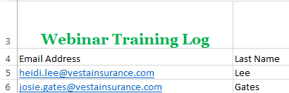   The realigned cell text

To change vertical text alignment:

1. Select the cell(s) you wish to modify.
   Selecting a cell
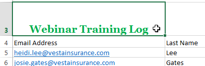
2. Select one of the three vertical alignment commands on the Home tab. In our example, we'll choose Middle Align.
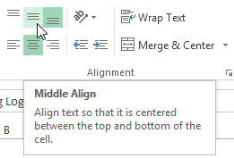   Choosing Middle Align
3. The text will realign.
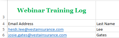   The realigned cell text

You can apply both vertical and horizontal alignment settings to any cell.

Cell borders and fill colors

Cell borders and fill colors allow you to create clear and defined boundaries for different sections of your worksheet. In our examples below, we'll add cell borders and fill color to our header cells to help distinguish them from the rest of the worksheet.

To add a border:

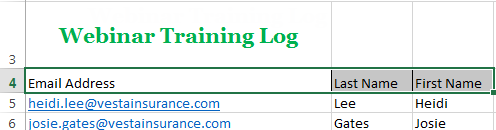
1. Select the cell(s) you wish to modify.
   Selecting a cell range
2. Click the drop-down arrow next to the Borders command on the Home tab. The Borders drop-down menu will appear.
3. Select the border style you want to use. In our example, we will choose to display All Borders.
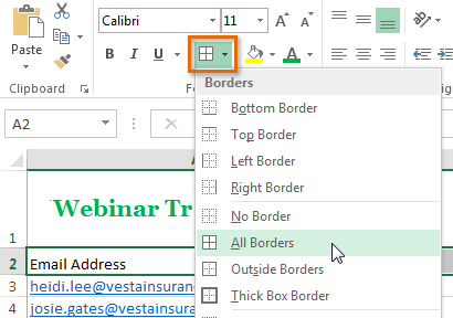   Choosing a border style
4. The selected border style will appear.
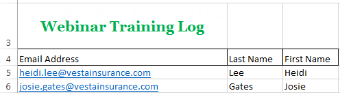   The added cell borders
   

You can draw borders and change the line style and color of borders with the Draw Borders tools at the bottom of the Borders drop-down menu.

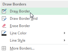Drawing custom borders

To add a fill color:

1. Select the cell(s) you wish to modify.
   Selecting a cell range
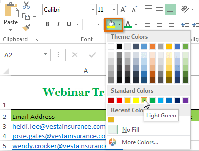
2. Click the drop-down arrow next to the Fill Color command on the Home tab. The Fill Color menu will appear.
3. Select the fill color you want to use. A live preview of the new fill color will appear as you hover the mouse over different options. In our example, we'll choose Light Green.
   Choosing a cell fill color
4. The selected fill color will appear in the selected cells.
   The new fill color

Cell styles

Rather than formatting cells manually, you can use Excel's predesigned cell styles. Cell styles are a quick way to include professional formatting for different parts of your workbook, such as titles and headers.

To apply a cell style:

In our example, we'll apply a new cell style to our existing title and header cells.

1. Select the cell(s) you wish to modify.
   Selecting a cell range
2. Click the Cell Styles command on the Home tab, then choose the desired style from the drop-down menu. In our example, we'll choose Accent 1.
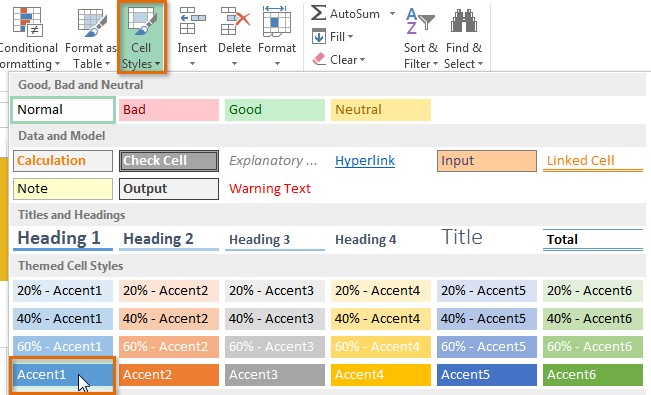   Choosing a cell style
3. The selected cell style will appear.
   
   The new cell style

Applying a cell style will replace any existing cell formatting except for text alignment. You may not want to use cell styles if you've already added a lot of formatting to your workbook.

Formatting text and numbers

One of the most powerful tools in Excel is the ability to apply specific formatting for text and numbers. Instead of displaying all cell content in exactly the same way, you can use formatting to change the appearance of dates, times, decimals, percentages (%), currency ($), and much more.

To apply number formatting:

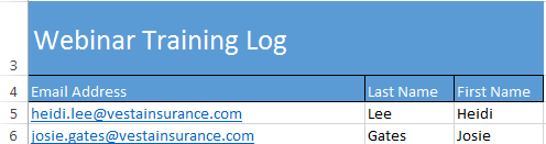
In our example, we'll change the number format for several cells to modify the way dates are displayed.

1. Select the cells(s) you wish to modify.
   
   Selecting a cell range
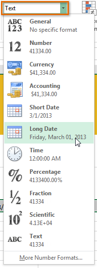
2. Click the drop-down arrow next to the Number Format command on the Home tab. The Number Formatting drop-down menu will appear.
3. Select the desired formatting option. In our example, we will change the formatting to Long Date.
   Choosing Long Date
   
4. The selected cells will change to the new formatting style. For some number formats, you can then use the Increase Decimal and Decrease Decimal commands (below the Number Format command) to change the number of decimal places that are displayed.
   The applied number formatting

Click the buttons in the interactive below to learn about different text and number formatting options.

General

General is the default format for any cell. When you enter a number into the cell, Excel will guess the number format that is most appropriate.

For example, if you enter "1-5", the cell will display the number as a Short Date, "1/5/2010".

Number

Number formats numbers with decimal places.

For example, if you enter "4" into the cell, the cell will display the number as "4.00".

Accounting

Accounting formats numbers as monetary values like the Currency format, but it also aligns currency symbols and decimal places within columns.

This format makes it easier to read long lists of currency figures.

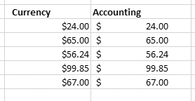
Currency

Currency formats numbers as currency with a currency symbol.

For example, if you enter "4" into the cell, the cell will display the number as "$4.00".

More Number Formats

You can easily customize any format in More Number Formats.

For example, you could change the U.S. dollar sign to another currency, have numbers display commas, change the number of displayed decimal places, etc.

Text

Text formats numbers as text, meaning that what you enter into the cell will appear exactly as it was entered.

Excel defaults to this setting if a cell contains both text and numbers.

Scientific

Scientific formats numbers in scientific notation.

For example, if you enter "140000" into the cell, then the cell will display the number as "1.40E+05".

Note: by default Excel will format the cell in scientific notation if it contains a large integer. If you do not want Excel to format large integers with scientific notation, use the Number format.

Fraction

Fraction formats numbers as fractions separated by the forward slash.

For example, if you enter "1/4" into the cell, the cell will display the number as "1/4". If you enter "1/4" into a cell that is formatted as General, the cell will display the number as a date, "4-Jan".

Percentage

Percentage formats numbers with decimal places and the percent sign.

For example, if you enter "0.75" into the cell, the cell will display the number as "75.00%".

Time

Time formats numbers as HH/MM/SS and notes AM or PM.

For example, "10:25:00 AM".

Long Date

Long Date formats numbers as Weekday, Month DD, YYYY.

For example, "Monday, August 14, 2013".

Short Date

Short Date formats numbers as M/D/YYYY.

For example, August 8th, 2013 would be "8/8/2013".

Challenge!

1. Open an existing Excel 2013 workbook. If you want, you can use our Lesson 9 Practice Workbook.
2. Select a cell and change the font style, size, and color of the text. If you are using the example, change the title in cell A3 to Verdana font style, size 16, with a font color of green.
3. Apply bold, italics, or underline to a cell. If you are using the example, bold the text in cell range A4:C4.
4. Try changing the vertical and horizontal text alignment for some cells.
5. Add a border to a cell range. If you are using the example, add a border to the header cells in in row 4.
6. Change the fill color of a cell range. If you are using the example, add a fill color to row 4.
7. Try changing the formatting of a number. If you are using the example, change the date formatting in cell range D4:H4 to Long Date.