Excel 2010
Using What-If Analysis
Introduction
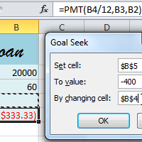
Imagine you're trying to solve a complicated problem with Excel. For example, you might need to calculate an unknown value. You could try solving it on your own, plugging in different numbers until you find the right answer. However, this method could take a lot of time and effort.
Instead of calculating the answer by yourself, you could use a powerful Excel tool called what-if analysis. This feature makes it easier to experiment with your data. In this lesson, we'll show you how to use what-if analysis to answer different kinds of questions.
What-if analysis
Excel includes many powerful tools to perform complex mathematical calculations, such as what-if analysis. This feature can help you experiment and answer questions with your data, even when the data is incomplete. In this lesson, you will learn how to use a what-if analysis tool called Goal Seek.
Goal Seek
Whenever you create a formula or function in Excel, you put various parts together to calculate a result. Goal Seek works in the opposite way: It lets you start with the desired result, and it calculates the input value that will give you that result. We'll use a few examples to show how to use Goal Seek.
To use Goal Seek (Example 1):
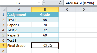
Imagine you're enrolled in a class. You currently have a grade of 65, and you need at least a 70 to pass the class. Luckily, you have one final assignment that might be able to raise your average. You can use Goal Seek to find out what grade you need on the final assignment to pass the class.
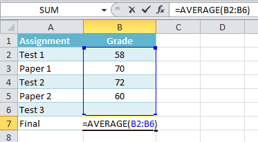
In the image below, you can see that the grades on the first four assignments are 58, 70, 72, and 60. Even though we don't know what the fifth grade will be, we can go ahead and write a formula or function that calculates the final grade. In this case, each assignment is weighted equally, so all we have to do is average all five grades by typing =AVERAGE(B2:B6). Once we use Goal Seek, cell B6 will show us the minimum grade we'll need to make on that assignment.
 Function calculating the monthly payment
- Select the cell whose value you wish to change. Whenever you use Goal Seek, you'll need to select a cell that already contains a formula or function. In our example, we'll select cell B7 because it contains the formula =AVERAGE(B2:B6).
 Selecting cell B7
 - From the Data tab, click the What-If Analysis command, then select Goal Seek from the drop-down menu.
 Selecting Goal Seek from the drop-down menu
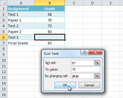
 - A dialog box will appear with three fields:
- Set cell: The cell that will contain the desired result. In our example, cell B7 is already selected.
- To value: The desired result. In our example, we'll enter 70 because we need to earn at least that to pass the class.
- By changing cell: The cell where Goal Seek will place its answer. In our example, we'll select cell B6, because we want to determine the grade we need to earn on the final assignment.
- When you're done, click OK.
 Entering the desired values into the dialog box and clicking OK
 - The dialog box will tell you if Goal Seek was able to find a solution. Click OK.
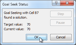 Clicking OK
 - The result will appear in the specified cell. In our example, Goal Seek calculated that we will need to score at least a 90 on the final assignment to earn a passing grade.
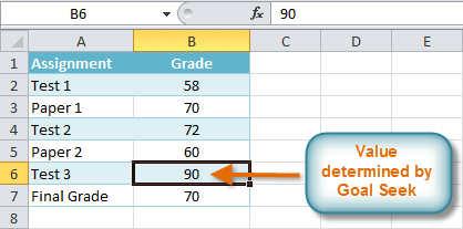 The completed Goal Seek and calculated value
To use Goal Seek (Example 2):
Suppose you need a loan to buy a new car. You already know you want a loan amount of $20,000, a 60-month term (the length of time it takes to pay off the loan), and a payment of no more than $400 per month. However, you're not sure yet what the interest rate is going to be.
In the image below, you can see that Interest Rate is left blank, and Payment is $333.33. That's because the payment is being calculated by a specialized function called the PMT (Payment) function, and $333.33 is what the monthly payment would be if there were no interest ($20,000 divided by 60 monthly payments).
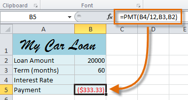 Function calculating the monthly payment
If we typed different values into the empty Interest Rate cell, we could eventually find the value that causes Payment to be $400, and that would be the highest interest rate that we could afford. However, Goal Seek can do this automatically by starting with the result and working backward.
To insert the PMT function:
- Select the cell where you want the function to be.
- From the Formula tab, select the Financial command.
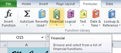 The Financial command
 - A drop-down menu will appear showing all finance-related functions. Scroll down and select the PMT function.
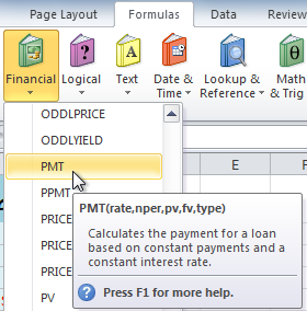 Selecting the PMT function
 - A dialog box will appear.
- Enter the desired values and/or cell references into the different fields. In this example, we're only using Rate, Nper (the number of payments), and Pv (the loan amount).
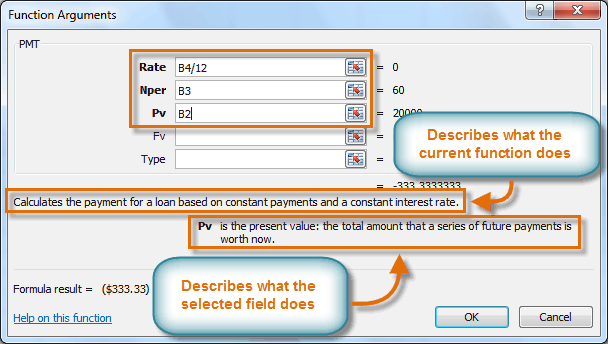 Entering values into the necessary fields
 - Click OK. The result will appear in the selected cell. Note that this is not our final result, as we still don't know what the interest rate will be.
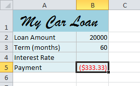 The monthly payment, not including interest
To use Goal Seek to find the interest rate:
Now that we've added the PMT function, we can use Goal Seek to find the interest rate we will need.
- From the Data tab, click the What-If Analysis command.
- Select Goal Seek.
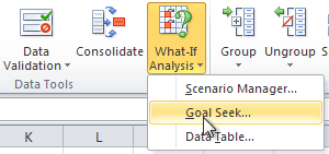 Selecting Goal Seek
 - A dialog box will appear containing three fields:
- Set cell: This is the cell that will contain the desired result (in this case, the monthly payment). In this example, we will set it to B5 (it doesn't matter whether it's an absolute or relative reference).
- To value: This is the desired result. We'll set it to -400. Since we're making a payment that will be subtracted from our loan amount, we have to enter the payment as a negative number.
- By changing cell: This is the cell where Goal Seek will place its answer (in this case, the interest rate). We'll set it to B4.
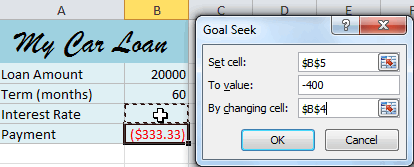 Entering values into the Goal Seek fields
 - When you're done, click OK. The dialog box will tell you whether or not Goal Seek was able to find a solution. In this example, the solution is 7.42%, and it has been placed in cell B4. This tells us that a 7.42% interest rate will give us a $400-per-month payment on a $20,000 loan that is paid off over five years, or 60 months.
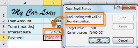 Solution found by Goal Seek
Other types of what-if analysis
For more advanced projects, you may want to consider the other types of what-if analysis: scenarios and data tables. Rather than starting from the desired result and working backward, like Goal Seek, these options allow you to test multiple values and see how the results change.
- Scenarios let you substitute values for multiple cells (up to 32) at the same time. You can create as many scenarios as you want and then compare them without changing the values manually. In the example below, each scenario contains a term and an interest rate. When each scenario is selected, it will replace the values in the spreadsheet with its own values, and the result will be recalculated.
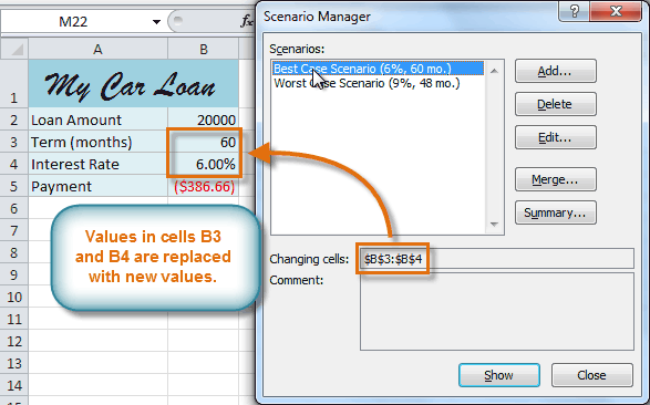 Using the Scenario Manager to compare different options
For more information about scenarios, check out this article from Microsoft.
- Data tables allow you to take one or two variables in a formula and replace them with as many different values as you want, then view the results in a table. This option is especially powerful because it shows multiple results at the same time, unlike scenarios or Goal Seek. In the example below, we can view 24 possible results for a car loan.
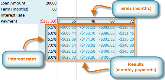 Data tables
For more information about data tables, check out this article from Microsoft.
Challenge!
- Open an existing Excel workbook. If you want, you can use this example.
- Use Goal Seek to determine an unknown value. If you're using the example, go to the History Class worksheet and use Goal Seek to determine what grade you would need on Test 3 to earn a final grade average of 90.
- Insert the PMT function into the worksheet. If you are using the example, go to the Car Loan worksheet and insert the function into cell B5.
- Use Goal Seek to find the interest rate you will need in order to have a monthly payment of $400. What interest rate would you need if you could only afford a $380 monthly payment?


