Excel 2010

Freezing worksheet panes

Video: Freezing Worksheet Panes in Excel 2010

Watch the video (1:50).

The ability to freeze specific rows or columns in your worksheet can be a useful feature in Excel. It is called freezing panes. When you freeze panes, you select rows or columns that will remain visible all the time, even as you are scrolling. This is particularly helpful when working with large spreadsheets.

To freeze rows:

1. Select the row below the rows you want frozen. For example, if you want rows 1 and 2 to always appear at the top of the worksheet even as you scroll, then select row 3.
   Selecting row 3
2. Click the View tab.
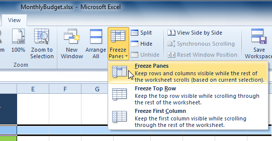
3. Click the Freeze Panes command. A drop-down menu appears.
4. Select Freeze Panes.
   Selecting the Freeze Panes command from the View tab
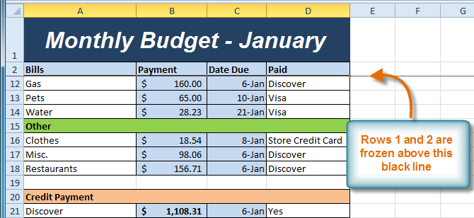
5. A black line appears below the rows that are frozen in place. Scroll down in the worksheet to see the rows below the frozen rows.
   Rows 1 and 2 are frozen

To freeze columns:

1. Select the column to the right of the columns you want frozen. For example, if you want columns A and B to always appear to the left of the worksheet even as you scroll, then select column C.
   Selecting column C
2. Click the View tab.
3. Click the Freeze Panes command. A drop-down menu appears.
4. Select Freeze Panes.
   Selecting the Freeze Panes command from the View tab
5. A black line appears to the right of the frozen area. Scroll across the worksheet to see the columns to the right of the frozen columns.
   Columns A and B are frozen

To unfreeze panes:

1. Click the View tab.
2. Click the Freeze Panes command. A drop-down menu appears.
3. Select Unfreeze Panes. The panes will be unfrozen, and the black line will disappear.
   Selecting the Unfreeze Panes command from the View tab