Excel 2007

Creating a PivotTable report

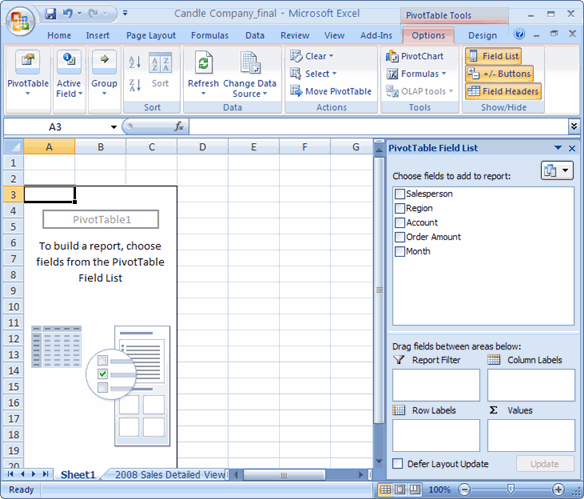
If you use the sample spreadsheet to create a PivotTable, you can see that the column headings are salesperson, region, account, order amount, and month. When you create a PivotTable, each column label in your data becomes a field that can be used in the report. The Field List appears on the right side of the report, while the layout area appears on the left.

To create a PivotTable report (Part 2):

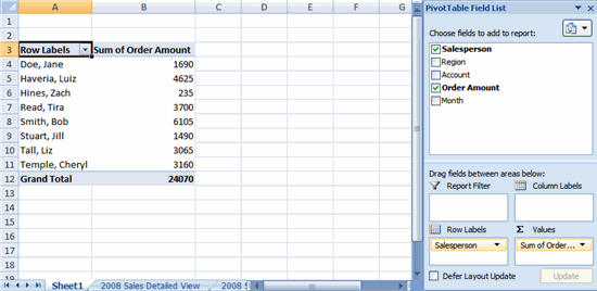
• Determine what question you want your PivotTable report to answer. For example, using the sample spreadsheet, you might want to know which salesperson sold the highest dollar amount.
• Determine the fields that are necessary to answer this question—in this example, salesperson and order amount.
• Select the check box next to the Salesperson field in the PivotTable Field List. The field will appear in the drag-and-drop area at the bottom of the field list and in the layout area. The order amount data appears on the right. This is a default setting in Excel—data with numbers will always appear on the right.
• Select the check box next to the Order Amount field in the PivotTable Field List. The field will appear in the drag-and-drop area at the bottom of the field list and in the layout area. All of the salesperson data appears on the left side as rows.
• You can now see the answer to your question in the report on the left.

If you change any of the data in your source worksheet, the PivotTable will not update automatically. To manually update it, select the PivotTable and then go to OptionsRefresh.

To add a report filter:

• Select a field in the Field List. In this example, choose Region. By default, it will appear in the Row Labels group.
• Click and drag Region into the Report Filter section.
• Release the mouse button. The region appears at the top of the report as a filter.
• The arrow by the Region fields shows (All). To show just the data for a specific region, click the drop-down arrow, and select the region. To see multiple regions, click the Multiple Regions box, select the regions to display, then click OK.