Excel 2007
Creating Pivot Tables
PivotTable reports
Watch the video! (10:41 min)
Download the example to work along with the video.
Why are they named PivotTables?
You may be wondering why it is called a PivotTable. Basically, PivotTables allow you to pivot, or move, data so you can produce answers to questions. Once you create a PivotTable, you can very easily see what effect pivoting the data has on the spreadsheet information.
To create a PivotTable report (Part I):
- Select the cells in your spreadsheet that you want to use in the PivotTable report.
- Select the Insert tab.
- Click the PivotTable command.
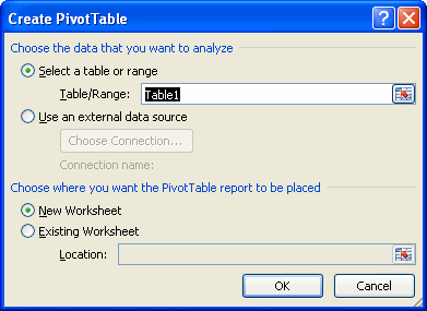
- Click PivotTable again. Excel selects cells in the actual spreadsheet, and the Create PivotTable dialog box opens.
- Select a table or range is already selected, and the Table/Range field shows the range of the selected data. New Worksheet is also selected by default as the place where the report will be placed.

- Click Existing Worksheet, then select a worksheet if you do not want the PivotTable to appear in a new worksheet.
- Click OK.


