Excel 2007

Freezing worksheet panes

The ability to freeze, or lock, specific rows or columns in your spreadsheet is a useful feature in Excel. It is called freezing panes. When you freeze panes, you select rows or columns that will remain visible all the time, even as you are scrolling. This is particularly useful when working with large spreadsheets.

To freeze a row:

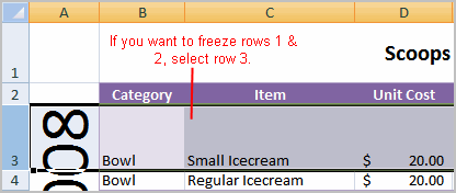
• Select the row below the one you want frozen. For example, if you want rows 1 and 2 to appear at the top even as you scroll, select row 3.

• Click the View tab.
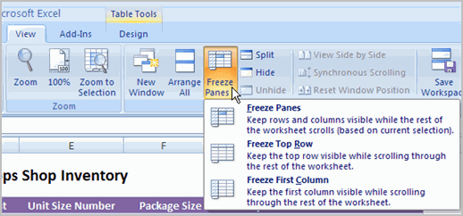
• Click the Freeze Pane command in the Window group.

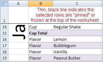
• Choose Freeze Panes. A thin, black line appears below everything that is frozen in place.

• Scroll down in the worksheet to see the pinned rows.

To unfreeze a pane:

• Click the Freeze Pane command.
• Select the Unfreeze command.

To freeze a column:

• Select the column to the right of the column(s) you want frozen. For example, if you want columns A and B to always appear on the left, select column C.
• Click the View tab.
• Click the Freeze Pane command in the Window group.
• Choose Freeze Pane. A thin, black line appears to the right of the frozen area.
• Scroll across in the worksheet to see the pinned columns.