3.2 Statistical IF Functions
Learning Objectives
- Use the COUNTIF function to count selected nonblank cells in a range based on one criteria argument.
- Use the AVERAGEIF function to calculate the average of selected cells in a range based on the values in an alternate range of cells and one criteria argument.
- Use the SUMIF function to calculate the sum of selected cells in a range based on the values in an alternate range of cells and one criteria argument.
- Use the COUNTIFS function to count selected nonblank cells in a range based on more than one criteria argument that utilizes a logical test.
- Use the AVERAGEIFS function to calculate the average of selected cells in a range based on the values in an alternate range of cells using more than one criteria argument that utilizes a logical test.
- Use the SUMIFS function to calculate the sum of selected cells in a range based on the values in an alternate range of cells using more than one criteria argument that utilizes a logical test.
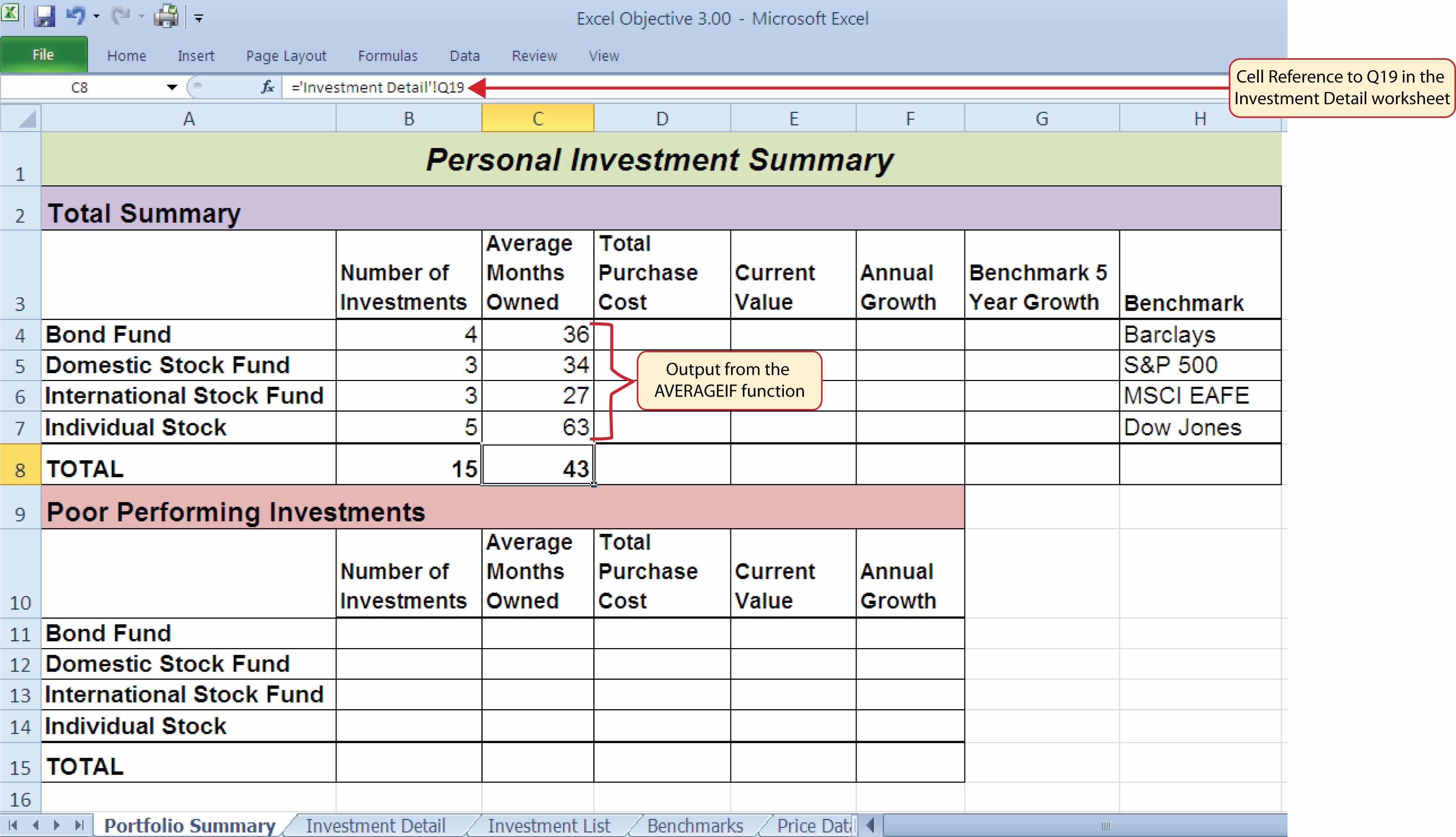
This section will demonstrate the use of statistical IF functions. Statistical IF functionsStatistical functions that provide the ability to evaluate the contents in a cell location before including it in a mathematical calculation. Cell locations can be selected from a range based on specific criteria or a logical test. provide you with the ability to evaluate the contents in a cell location before including them in a mathematical calculation. This allows you to selectively include targeted cell locations when executing statistical calculations such as sum, average, count, and so on. We will use several statistical IF functions to construct the Portfolio Summary worksheet shown in Figure 3.1 "Completed Personal Investment Portfolio Workbook", which contains two main sections. The Total Summary section (Rows 2 through 8) shows an overview for all investments in the portfolio by investment type. This will allow us to compare the growth performance among the Bond Funds, Domestic Stock Funds, and others. The Poor Performing Investments section (Rows 9 through 15) will provide an overview of poor performing investments by investment type. For the purposes of this exercise, we will define a poor performing investment as one where the growth rate is below the target growth rate by more than 1% (see Column W on the Investment Detail worksheet). The statistical IF functions will allow us to establish criteria to select targeted investments that can be included in the calculations for each section of the Portfolio Summary worksheet.
The COUNTIF Function
Follow-along file: Continue with Excel Objective 3.00. (Use file Excel Objective 3.08 if starting here.)
Lesson Video: COUNTIF Function
The COUNTIF function differs from the regular COUNT function in two ways. First, the regular COUNT function counts only the number of cells in a range that contain numeric data. The COUNTIF function counts the number of cells in a range that contain numeric or text data. Second, the COUNTIF function allows you to selectively count the cells in a range based on specific criteria.
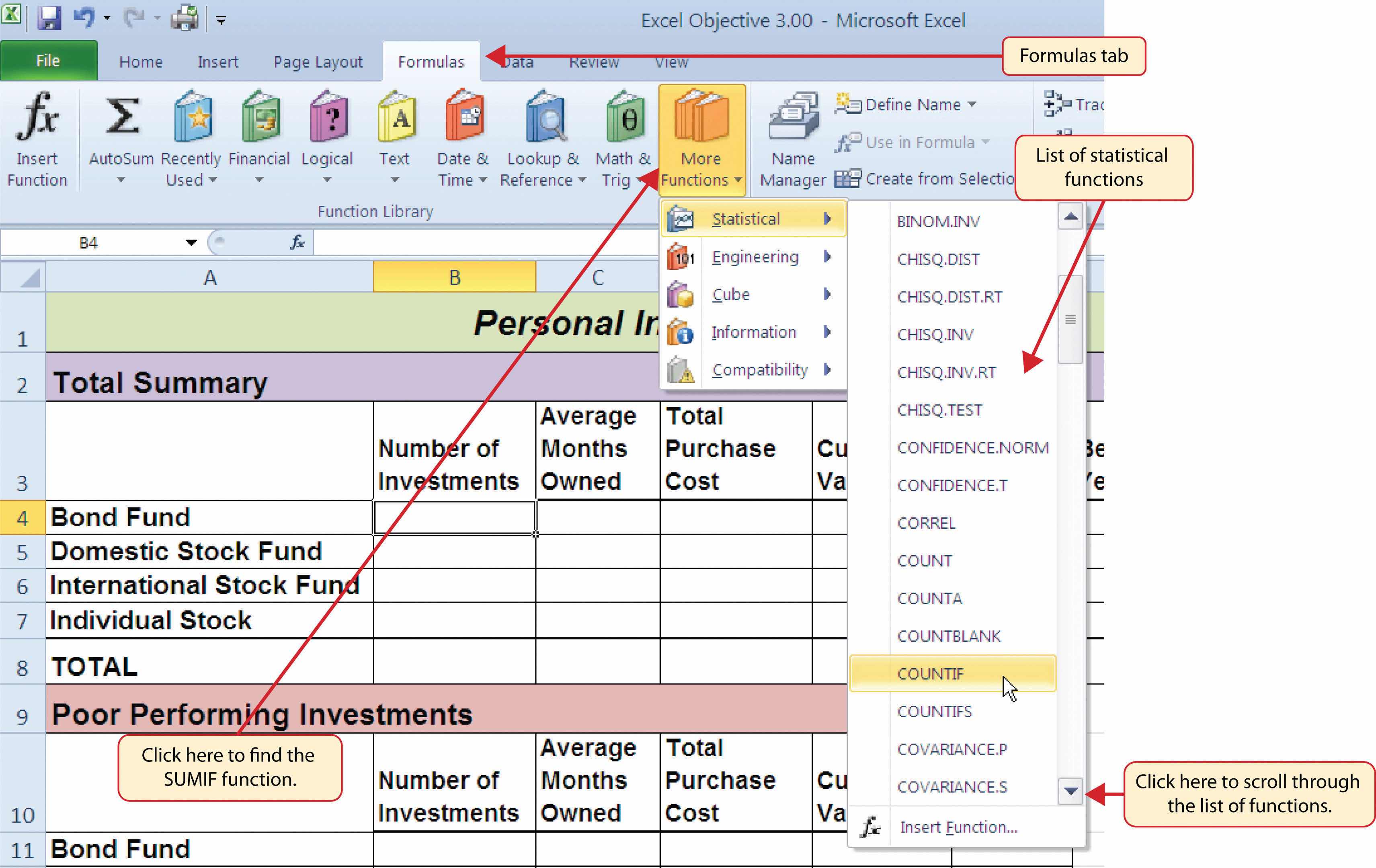
The COUNTIF function contains two arguments: range and criteria. The range argument is defined with the range of cells that will be counted. The criteria argument is defined with the criteria that will be used to decide if a cell in the range should be included in the output of the function. The following steps explain how we can use the COUNTIF function to calculate the number of investments by investment type on the Portfolio Summary worksheet:
- Click cell B4 on the Portfolio Summary worksheet.
- Click the Formulas tab of the Ribbon.
- Click the More Functions button in the Function Library group of commands.
- Place the mouse pointer over the Statistical option from the drop-down list.
- Click the scroll down arrow on the second drop-down list to find the COUNTIF function (see Figure 3.25 "Selecting the COUNTIF Function from the Function Library").
-
Click the COUNTIF function. This will open the Function Arguments dialog box.
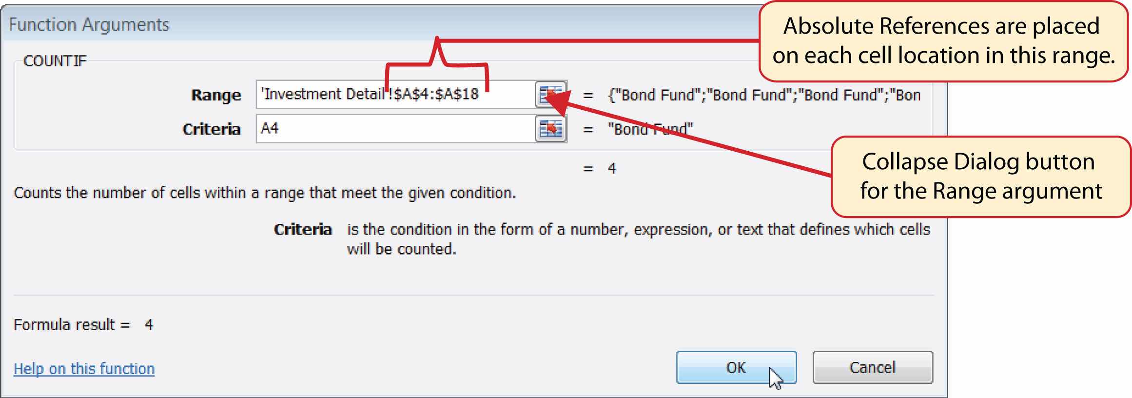
- Click the Collapse Dialog button next to the Range argument on the Function Arguments dialog box (see Figure 3.26 "Completed Function Arguments Dialog Box for the COUNTIF Function").
- Click the Investment Detail worksheet tab.
- Highlight the range A4:A18 on the Investment Detail worksheet and press the ENTER key on your keyboard.
- Click in the Range argument input box and place an absolute reference on the range A4:A18. This is done by typing a dollar sign ($) in front of the column letter and row number for both cells in the range. Alternatively, place the insertion point after the 4 in cell reference A4 and press the F4 key on your keyboard. Then place the insertion point after the 8 in cell reference A18 and press the F4 key. This will add the $ to the appropriate positions automatically.
- Press the TAB key on your keyboard to advance to the next argument, which is the Criteria argument. Then type the cell location A4. The criteria for the function will be the investment type entered into cell A4 on the Portfolio Summary worksheet.
-
Click the OK button at the bottom of the Function Arguments dialog box. Figure 3.26 "Completed Function Arguments Dialog Box for the COUNTIF Function" shows the completed Function Arguments dialog box for the COUNTIF function. Notice the absolute references that were placed on each cell location in the range that was used to define the Range argument. The Criteria argument is defined with the cell A4, which means the function will only count cell locations in the range A4:A18 where the contents in the cell match the contents in cell A4.
- Copy the function in cell B4 and paste it into the range B5:B7 using the Paste Formulas command.
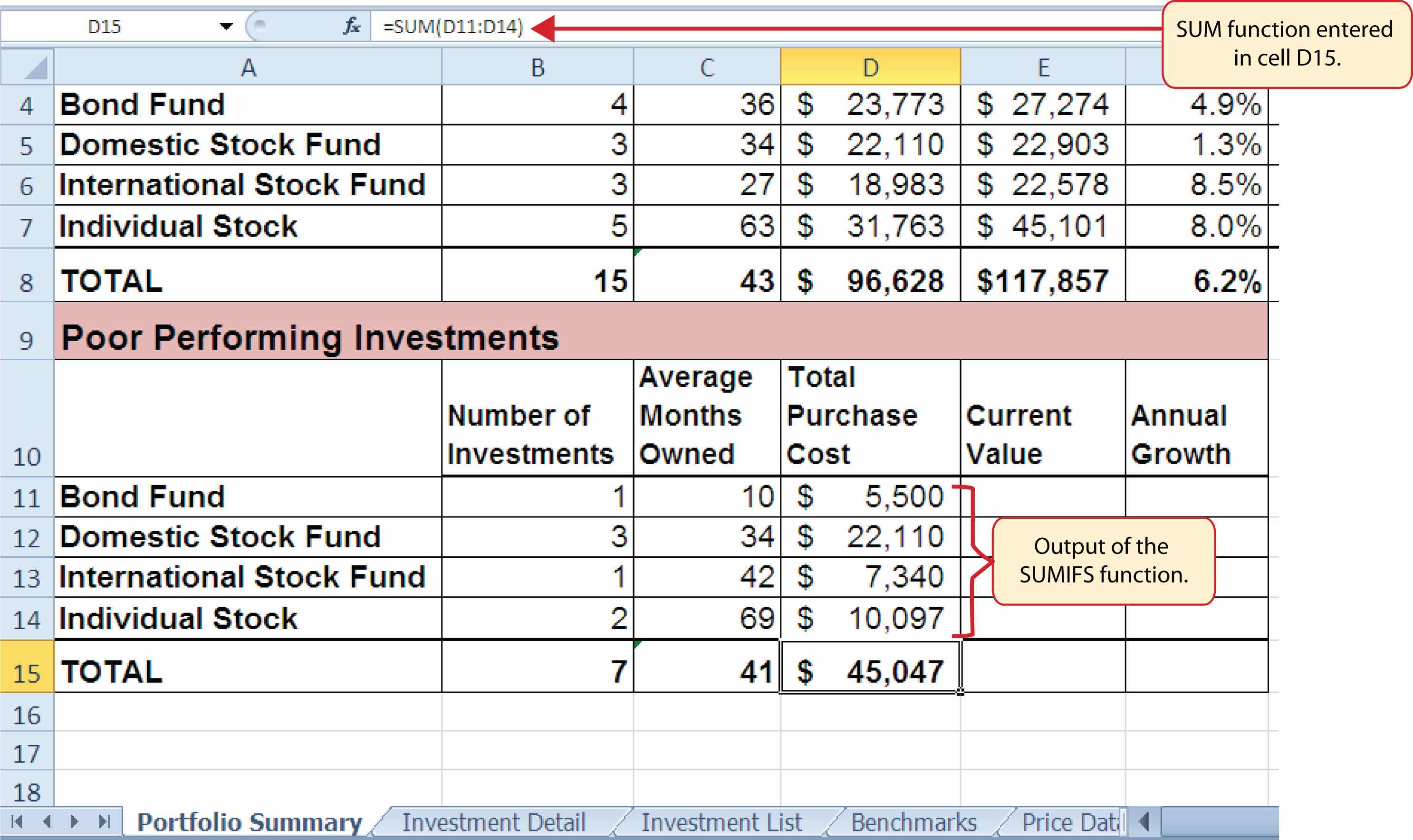
- Enter a SUM function in cell B8 that sums the values in the range B4:B7.
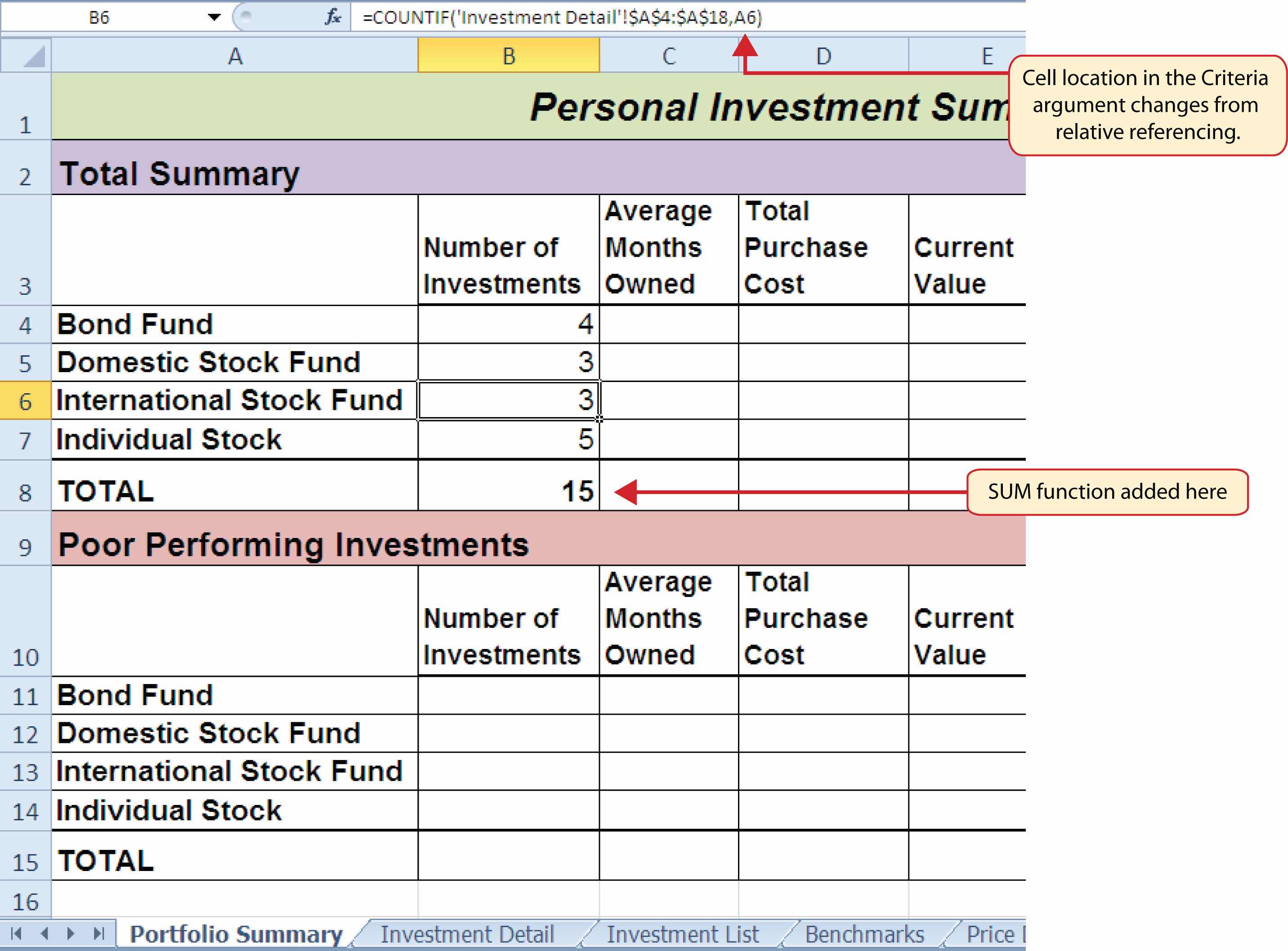
Figure 3.27 "COUNTIF Function Output in the Portfolio Summary Worksheet" shows the results of the COUNTIF function after it is pasted into the range B5:B7. Because of relative referencing, the cell location used in the criteria argument is changed after the function is pasted into the range B5:B7. For example, in cell B6, the function is counting the cell locations in the range A4:A18 where the contents match the contents of cell A6. This allows you to use the function to count the number of investments per investment type. As shown in the figure, the range B4:B7 now shows the number of investments in this portfolio by investment type.
Skill Refresher: COUNTIF Function
- Type an equal sign (=).
- Type the function name COUNTIF followed by an open parenthesis (().
- Define the range argument with a range of cells that will be counted.
- Type a comma.
- Define the criteria argument with a cell location, number, text, or logical test. Text and logical tests must be enclosed in quotation marks.
- Type a closing parenthesis ()).
- Press the ENTER key on your keyboard.
The AVERAGEIF Function
Follow-along file: Continue with Excel Objective 3.00. (Use file Excel Objective 3.09 if starting here.)
Lesson Video: AVERAGEIF Function
The AVERAGEIF function performs the identical mathematical calculation as the regular AVERAGE function. However, similar to the COUNTIF function, it allows you to define criteria that will select cells in a range that will be used in the function output. The AVERAGEIF function differs from the COUNTIF function in that it allows you to define two cell ranges instead of one. The first range pertains to the criteria that will be used to select cells for the function output. The second range contains the values that will be used to calculate the arithmetic mean. Table 3.8 "Arguments for the AVERAGEIF and SUMIF Functions" provides definitions for the arguments contained in the AVERAGEIF and SUMIF functions.
Table 3.8 Arguments for the AVERAGEIF and SUMIF Functions
| Argument |
Definition |
| Range |
Range of cells that will be evaluated by the criteria argument. |
| Criteria |
Criteria that will be used to evaluate the range of cells that is used to define the Range argument. This argument can be defined with a cell location, formula, number, text, or logical test. Note that text and logical tests must be enclosed in quotation marks. |
| [Average_range] or [Sum_range] |
Range of cells that will be used to calculate the average when using the AVERAGEIF function, or the sum when using the SUMIF function. This argument is enclosed in brackets because it does not always need to be defined. If this argument is omitted, the function will use the range of cells in the Range argument to calculate the output. |
The AVERAGEIF function will be used in the Portfolio Summary worksheet to calculate the average length of time that investments for each investment type are held. The following steps explain how to add this function to the worksheet:
- Click cell C4 on the Portfolio Summary worksheet.
- Click the Formulas tab on the Ribbon.
- Click the More Functions button in the Function Library group of commands.
- Place the mouse pointer over the Statistical option from the drop-down list (see Figure 3.25 "Selecting the COUNTIF Function from the Function Library").
- Click the AVERAGEIF function, which will be near the top of the list of functions. This opens the Function Arguments dialog box.
- Click the Collapse Dialog button next to the Range argument on the Function Arguments dialog box (see Figure 3.28 "Defined Arguments for the AVERAGEIF Function").
- Click the Investment Detail worksheet tab.
- Highlight the range A4:A18 on the Investment Detail worksheet and press the ENTER key on your keyboard.
- Click in the Range argument input box and place an absolute reference on the range A4:A18. This is done by typing a dollar sign ($) in front of the column letter and row number for both cells in the range.
- Press the TAB key on your keyboard to advance to the Criteria argument and type the cell location A4. The criteria for the function will be the investment type entered into cell A4 on the Portfolio Summary worksheet.
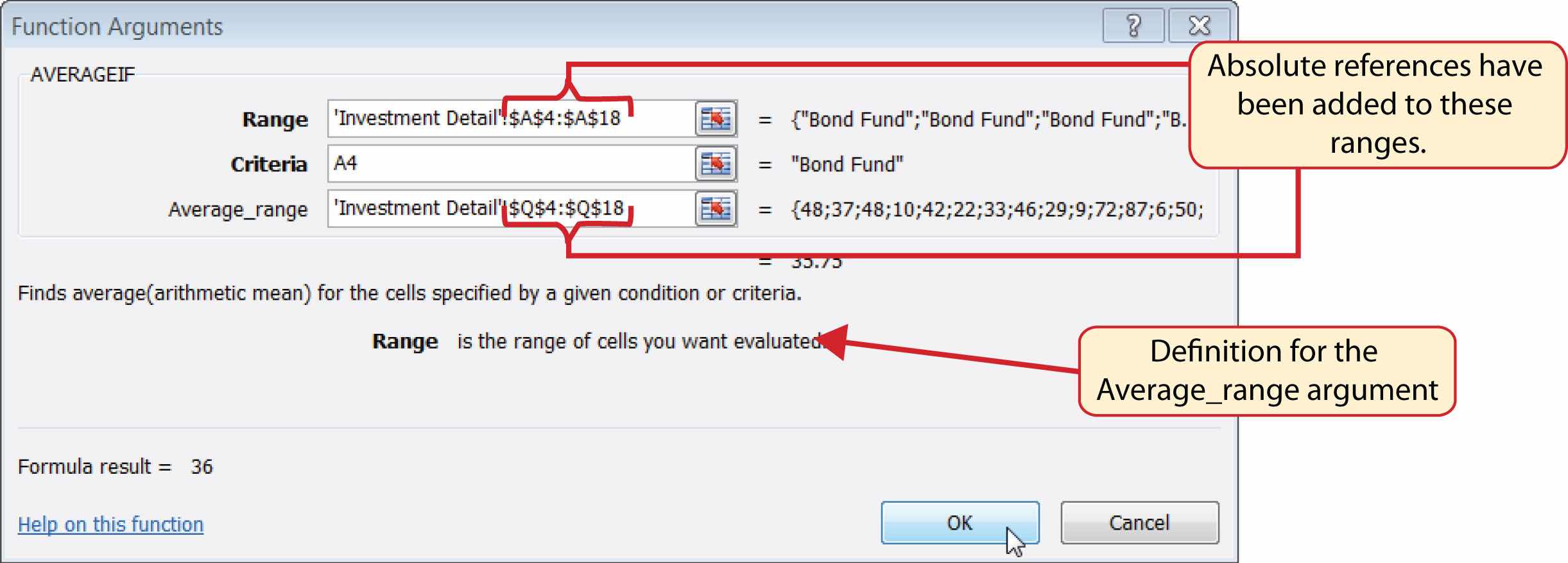
- Click the Collapse Dialog button next to the Average_range argument on the Function Arguments dialog box (see Figure 3.28 "Defined Arguments for the AVERAGEIF Function").
- Click the Investment Detail worksheet tab.
- Highlight the range Q4:Q18 on the Investment Detail worksheet and press the ENTER key on your keyboard.
- Click in the Average_range argument input box and place an absolute reference on the range Q4:Q18. This is done by typing a dollar sign ($) in front of the column letter and row number for both cells in the range.
-
Click the OK button at the bottom of the Function Arguments dialog box.
Figure 3.28 "Defined Arguments for the AVERAGEIF Function" shows the Function Arguments dialog box for the AVERAGEIF function that will be input into cell C4. Notice that absolute references are placed on the cell locations used to define the Range and Average_range arguments. The function will evaluate the cells in the range A4:A18 using the value that exists in cell A4 on the Portfolio Summary worksheet. When a cell in the range A4:A18 meets the criteria, the function will pull the cell location in the same row from the range Q4:Q18 and include it in the average calculation.
- Copy the function in cell C4 and paste it into the range C5:C7 using the Paste Formulas option.
- Type an equal sign (=) in cell C8.
- Click the Investment Detail worksheet tab. Then click cell Q19 and press the ENTER key on your keyboard.
Figure 3.29 "AVERAGEIF Function Output on the Portfolio Summary Worksheet" shows the output of the AVERAGEIF function in the Average Months Owned column on the Portfolio Summary worksheet. The function calculates the average months owned in Column Q on the Investment Detail worksheet where the investment type is equal to the description entered in the range A4:A7 on the Portfolio Summary worksheet.
Integrity Check
Matching Row Numbers for the Range and Average_range (or Sum_range) Arguments
When defining the Average_range argument for the AVERAGEIF function or the Sum_range argument for the SUMIF function, it is good practice to make sure the row numbers match the row numbers used in the Range argument. For example, if the Range argument is defined with the range A4:A12, the range used to define the Average_range or Sum_range argument should begin with Row 4 and end with Row 12. If the row numbers in these two arguments do not match, Excel will include the values only in the rows used to define the Range argument. For example, if the Range argument is defined with the range A4:A12 and the Average_range (or Sum_range) argument is defined with the range D4:D20, only the values in cells D4:D12 will be included in the function output.
Skill Refresher: AVERAGEIF Function
- Type an equal sign (=).
- Type the function name AVERAGEIF followed by an open parenthesis (().
- Define the range argument with a range of cells that will be evaluated using the criteria argument.
- Type a comma.
- Define the criteria argument with a cell location, number, text, or logical test. Text and logical tests must be enclosed in quotation marks.
- Type a comma.
- Define the Average_range argument with a range that contains values to be averaged. Excel will use the range argument to calculate the average if this argument is omitted.
- Type a closing parenthesis ()).
- Press the ENTER key on your keyboard.
The SUMIF Function
Follow-along file: Continue with Excel Objective 3.00. (Use file Excel Objective 3.10 if starting here.)
Lesson Video: SUMIF Function
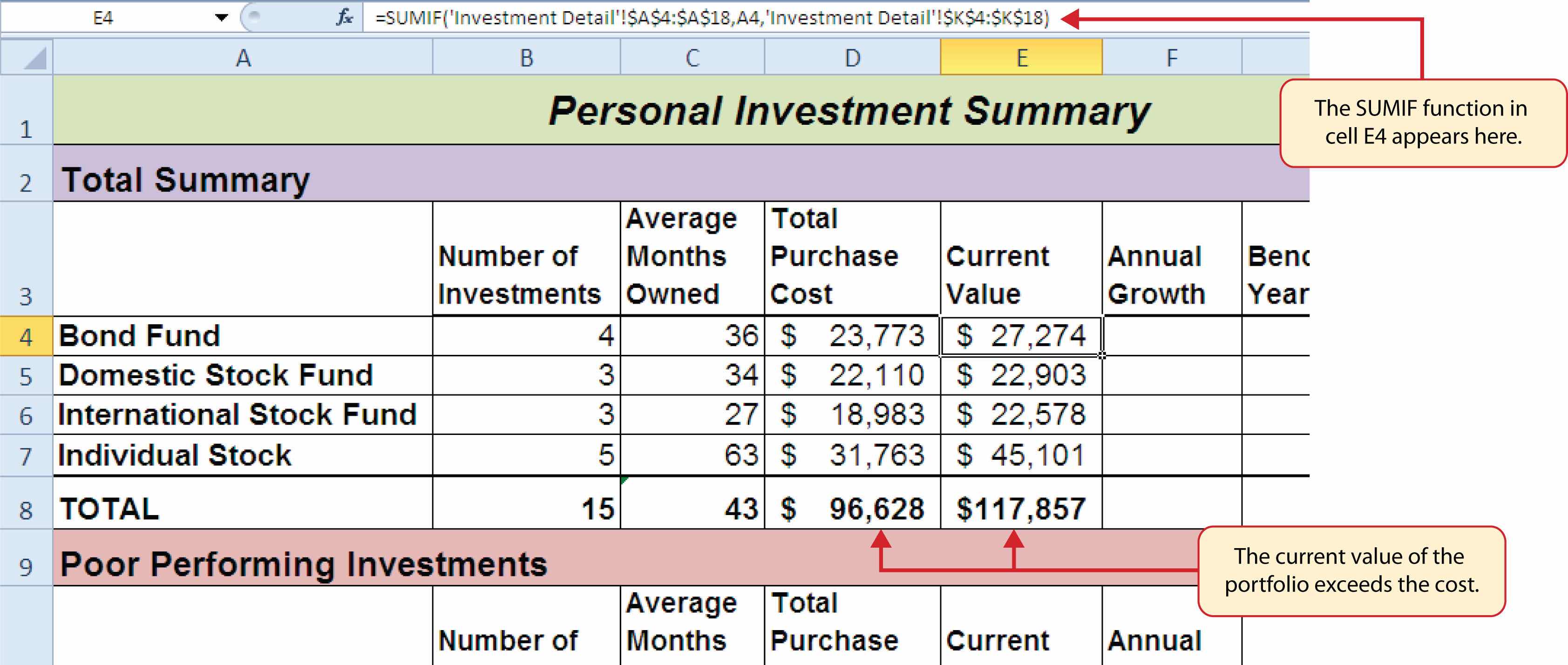
The SUMIF function performs the same mathematical calculation as the regular SUM function. However, similar to the AVERAGEIF function, this function allows you to select specific cells from a range that will be used in the output. The arguments for the SUMIF function are identical to the AVERAGEIF function (see Table 3.8 "Arguments for the AVERAGEIF and SUMIF Functions"). We will use the SUMIF function in two columns on the Portfolio Summary worksheet. The first column will show the total investment cost for each investment type. The second column will show the total current value for each investment type. This will allow us to calculate the total annual growth rate for each investment type. The following steps explain how we will use this function to complete the first column:
- Click cell D4 on the Portfolio Summary worksheet.
- Click the Formulas tab on the Ribbon.
- Click the Math & Trig button in the Function Library group of commands (see Figure 3.25 "Selecting the COUNTIF Function from the Function Library").
- Select the SUMIF function from the drop-down list. Use the scroll bar to scroll down to find the SUMIF function.
- Click the Collapse Dialog button next to the Range argument on the Function Arguments dialog box (see Figure 3.30 "Defined Arguments for the First SUMIF Function on the Portfolio Summary Worksheet").
- Click the Investment Detail worksheet tab.
- Highlight the range A4:A18 on the Investment Detail worksheet and press the ENTER key on your keyboard.
- Click in the Range argument input box and place an absolute reference on the range A4:A18. This is done by typing a dollar sign ($) in front of the column letter and row number for both cells in the range.
- Press the TAB key on your keyboard to advance to the Criteria argument and type the cell location A4. The criteria for the function will be the investment type entered into cell A4 on the Portfolio Summary worksheet.
-
Click the Collapse Dialog button next to the Sum_range argument on the Function Arguments dialog box (see Figure 3.30 "Defined Arguments for the First SUMIF Function on the Portfolio Summary Worksheet").
- Click the Investment Detail worksheet tab.
- Highlight the range G4:G18 on the Investment Detail worksheet and press the ENTER key on your keyboard.
- Click in the Sum_range argument input box and place an absolute reference on the range G4:G18. This is done by typing a dollar sign ($) in front of the column letter and row number for both cells in the range.
- Click the OK button at the bottom of the Function Arguments dialog box.
- Copy the function in cell D4 and paste it into the range D5:D7 using the Paste Formulas option.
- Enter a regular SUM function into cell D8 on the Portfolio Summary worksheet to calculate the sum of the values in the range D4:D7.
Figure 3.30 "Defined Arguments for the First SUMIF Function on the Portfolio Summary Worksheet" shows how the SUMIF arguments were defined for the Total Purchase Cost column on the Portfolio Summary worksheet. Notice that the row numbers are identical in the range used to define the Range argument and the Sum_range argument.
The following steps explain how to add the SUMIF function to the second column on the Portfolio Summary worksheet:
- Click cell E4 on the Portfolio Summary worksheet.
- Click the Formulas tab on the Ribbon.
- Click the Math & Trig button in the Function Library group of commands (see Figure 3.25 "Selecting the COUNTIF Function from the Function Library").
- Select the SUMIF function from the drop-down list. Use the scroll bar to scroll down to find the SUMIF function.
- Click the Collapse Dialog button next to the Range argument on the Function Arguments dialog box (see Figure 3.30 "Defined Arguments for the First SUMIF Function on the Portfolio Summary Worksheet").
- Click the Investment Detail worksheet tab.
- Highlight the range A4:A18 on the Investment Detail worksheet and press the ENTER key on your keyboard.
- Click in the Range argument input box and place an absolute reference on the range A4:A18. This is done by typing a dollar sign ($) in front of the column letter and row number for both cells in the range.
- Press the TAB key on your keyboard to advance to the Criteria argument and type the cell location A4.
- Click the Collapse Dialog button next to the Sum_range argument on the Function Arguments dialog box (see Figure 3.30 "Defined Arguments for the First SUMIF Function on the Portfolio Summary Worksheet").
- Click the Investment Detail worksheet tab.
- Highlight the range K4:K18 on the Investment Detail worksheet and press the ENTER key on your keyboard.
- Click in the Sum_range argument input box and place an absolute reference on the range K4:K18. This is done by typing a dollar sign ($) in front of the column letter and row number for both cells in the range.
- Click the OK button at the bottom of the Function Arguments dialog box.
- Copy the function in cell E4 and paste it into the range E5:E7 using the Paste Formulas option.
- Enter a regular SUM function into cell E8 on the Portfolio Summary worksheet to calculate the sum of the values in the range E4:E7.
Figure 3.31 "SUMIF Function Outputs in the Portfolio Summary Worksheet" shows the results of the SUMIF function in the Total Purchase Cost and Current Value columns in the Portfolio Summary worksheet.
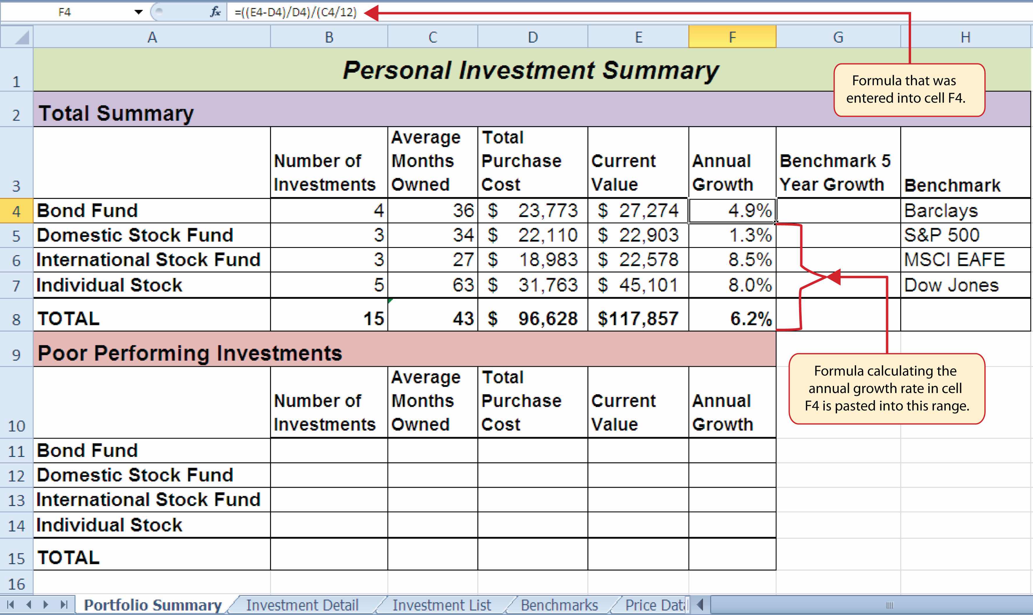
A formula can now be added to show the annual growth for each investment category. The following steps explain how to add this formula to the Portfolio Summary worksheet:
- Click cell F4 on the Portfolio Summary worksheet.
- Type an equal sign (=) followed by two open parenthesis ((().
- Click cell E4 and type a minus sign (−).
- Click cell D4 and type a closing parenthesis ()).
- Type a slash (/) for division and click cell D4.
- Type a closing parenthesis ()). This completes the first part of the formula, which is calculating the growth rate between the Total Purchase Cost (cell D4) and the Current Value (cell E4).
- Type a slash (/) for division followed by an open parenthesis (().
- Click cell C4, which is the Average Months Owned.
- Type a slash (/) for division and the number 12. This part of the formula converts the number of months owned to years by dividing it by 12. This result is being divided into the growth rate, which will then show the average growth per year.
- Type a closing parenthesis ()) and press the ENTER key on your keyboard.
- Copy the formula in cell F4 and paste it into the range F5:F8 using the Paste Formulas command.
Figure 3.32 "Completed Annual Growth Column in the Portfolio Summary Worksheet" shows the results of the statistical IF functions that were added to the Total Summary section of the Portfolio Summary worksheet. The statistical IF functions used on this worksheet allowed us to group the details in the Investment Detail worksheet by investment type. Once this was accomplished, we added a formula to show the annual growth rate by investment type.
Skill Refresher: SUMIF Function
- Type an equal sign (=).
- Type the function name SUMIF followed by an open parenthesis (().
- Define the range argument with a range of cells that will be evaluated using the criteria argument.
- Type a comma.
- Define the criteria argument with a cell location, number, text, or logical test. Text and logical tests must be enclosed in quotation marks.
- Type a comma.
- Define the Sum_range argument with a range that contains values to be summed. Excel will use the range argument to calculate the sum if this argument is omitted.
- Type a closing parenthesis ()).
- Press the ENTER key on your keyboard.
The COUNTIFS Function
Follow-along file: Continue with Excel Objective 3.00. (Use file Excel Objective 3.11 if starting here.)
Lesson Video: COUNTIFS Function
Up to this point, the statistical IF functions that were demonstrated provided the ability to define one criteria or logical test used to select cells from a targeted range. The next set of statistical functions that will be demonstrated provides the ability to define multiple sets of criteria for selecting cells from a targeted range. We will begin with the COUNTIFS function.
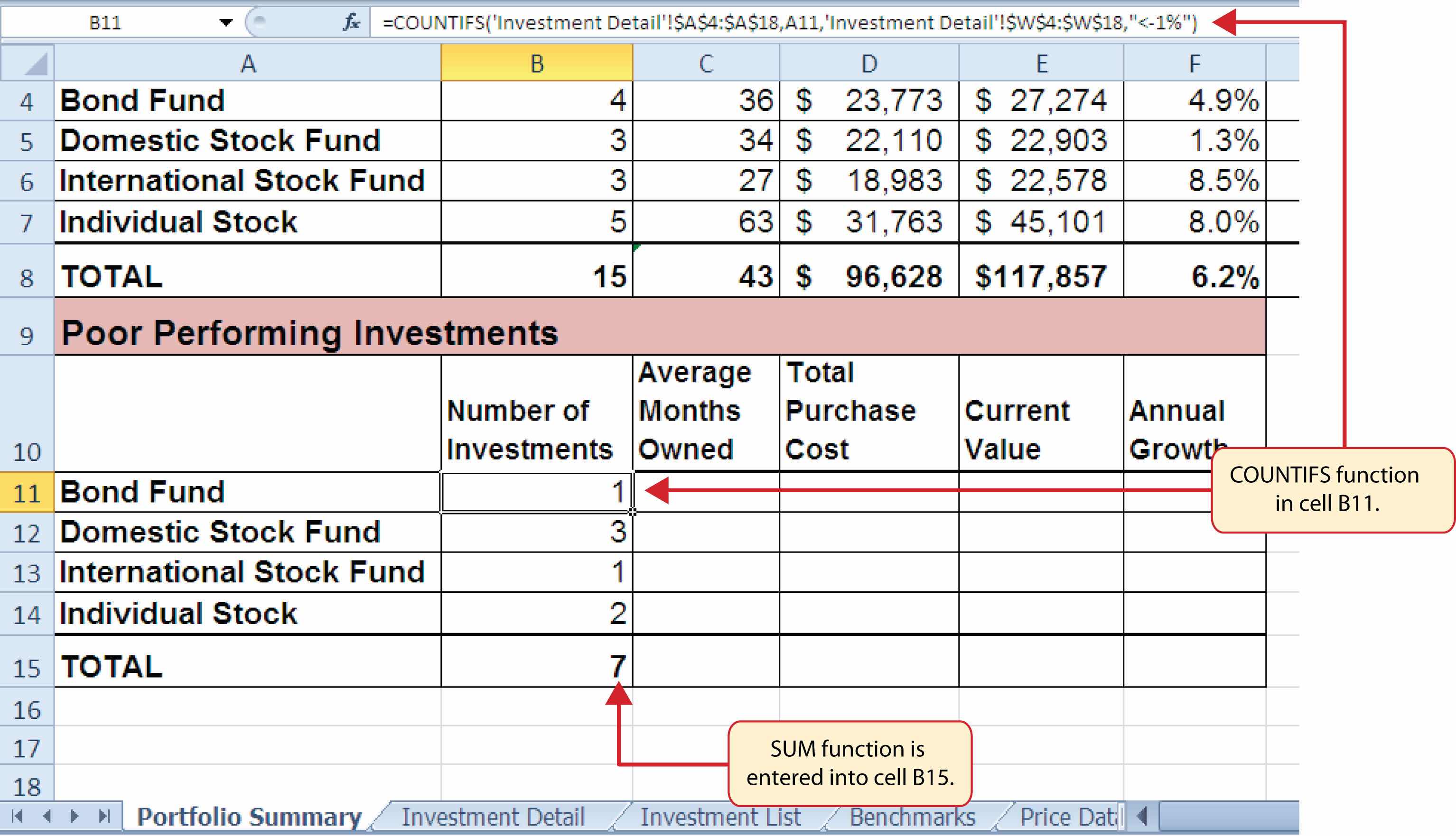
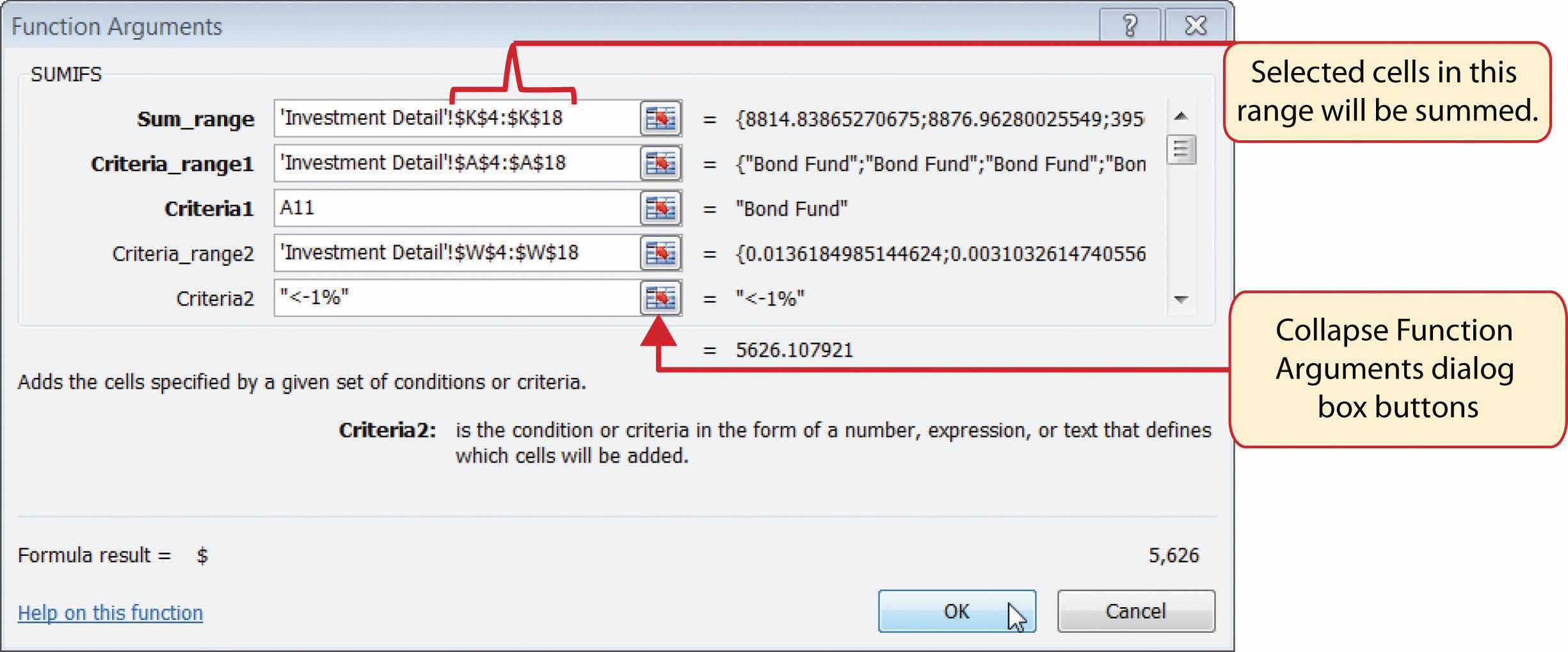
It is easy to distinguish the difference between a statistical IF function that allows one criteria argument to be defined and one that allows multiple criteria arguments. If the IF at the end of the function name is plural, you can define multiple sets of criteria arguments. Therefore, the COUNTIFS function provides the option of defining multiple sets of criteria for selecting cells from a targeted range that will be used in the function output. The arguments for the COUNTIFS function are established in pairs. For example, the first arguments for the function are Criteria_range1 and Criteria1. The function will use the Criteria1 argument to select cells in the Criteria_range1 argument. A second pair of arguments, Criteria_range2 and Criteria2, can be defined to select a subset of cell locations that were selected in the Criteria_range1 and Criteria1 arguments. This process can be repeated for several pairs of criteria arguments. We will continue to work on the Portfolio Summary worksheet by adding the COUNTIFS function to count the number of poor performing investments by investment type. The following steps explain how to add this function to the worksheet:
- Click cell B11 on the Portfolio Summary worksheet.
- Click the Formulas tab of the Ribbon.
- Click the More Functions button in the Function Library group of commands.
- Place the mouse pointer over the Statistical option from the drop-down list.
- Click the scroll down arrow on the second drop-down list to find the COUNTIFS function (see Figure 3.25 "Selecting the COUNTIF Function from the Function Library").
- Click the COUNTIFS function. This will open the Function Arguments dialog box.
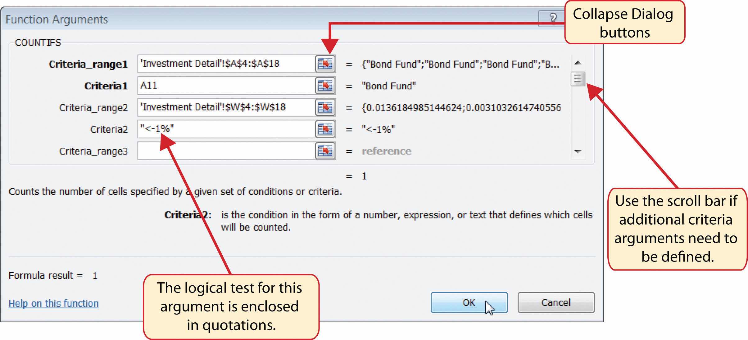
- Click the Collapse Dialog button next to the Criteria_range1 argument on the Function Arguments dialog box (see Figure 3.33 "Defined Arguments for the COUNTIFS Function").
- Click the Investment Detail worksheet tab.
- Highlight the range A4:A18 on the Investment Detail worksheet and press the ENTER key on your keyboard.
- Click in the Criteria_range1 argument input box and place an absolute reference on the range A4:A18. This is done by typing a dollar sign ($) in front of the column letter and row number for both cells in the range.
- Press the TAB key on your keyboard to advance to the Criteria1 argument and type the cell location A11. The criteria for the function will be the investment type that is entered into cell A11 on the Portfolio Summary worksheet. You will notice that when you define this argument, the Criteria_range2 argument will appear on the Function Arguments dialog box.
- Click the Collapse Dialog button next to the Criteria_range2 argument on the Function Arguments dialog box (see Figure 3.33 "Defined Arguments for the COUNTIFS Function").
- Click the Investment Detail worksheet tab.
- Highlight the range W4:W18 on the Investment Detail worksheet and press the ENTER key on your keyboard.
- Click in the Criteria_range2 argument input box and place an absolute reference on the range W4:W18. This is done by typing a dollar sign ($) in front of the column letter and row number for both cells in the range.
- Press the TAB key on your keyboard to advance to the Criteria2 argument.
- Type an open quotation mark followed by the logical test <−1% and then type a closing quotation mark (“<−1%”). The second criterion for this function is a logical test that will identify cell locations where the value is less than −1%. For the purposes of this exercise, a poor performing investment is one that is below the target growth rate by more than 1%.
- Click the OK button at the bottom of the Function Arguments dialog box.
- Copy the function in cell B11 and paste it into the range B12:B14 using the Paste Formulas command.
- Enter a SUM function in cell B15 on the Portfolio Summary worksheet that sums the values in the range B11:B14.
Why?
Use Statistical IF Functions for a Summary Worksheet
When creating a summary worksheet that summarizes detailed data from other worksheets, such as the Portfolio Summary worksheet in Figure 3.32 "Completed Annual Growth Column in the Portfolio Summary Worksheet", it is best to use statistical IF functions. If data is added to the detailed worksheet that is being summarized, the statistical IF functions will automatically include the new data in the summary worksheet. For example, suppose a row is added below Row 7 on the Investment Detail worksheet (see Figure 3.24 "Conditional Format Applied to the Range S4:T18") and another bond investment is added. The statistical IF functions will automatically pick up the new investment and include it in the Portfolio Summary worksheet. If regular statistical functions or formulas are used, the summary worksheet can easily become inaccurate if new data is added to the detailed worksheet or if the sort order is changed.
Figure 3.33 "Defined Arguments for the COUNTIFS Function" shows the completed arguments for the COUNTIFS function in the Function Arguments dialog box. Notice the scroll bar that appears on the right side of the Function Arguments dialog box. This allows you to scroll through and define multiple pairs of criteria arguments for the function.
Figure 3.34 "Outputs for the COUNTIFS Functions" shows the output of the COUNTIFS function on the Portfolio Summary worksheet. The criteria established for the COUNTIFS function shows that there are a total of seven investments that are underperforming in the portfolio.
Skill Refresher: COUNTIFS Function
- Type an equal sign (=).
- Type the function name COUNTIFS followed by an open parenthesis (().
- Define the Criteria_range1 argument with a range of cells that will be counted.
- Type a comma.
- Define the Criteria1 argument with a cell location, number, text, or logical test. Text and logical tests must be enclosed in quotation marks. This argument will be used to select cells from the Criteria_range1 argument.
- Type a comma and then repeat steps 3, 4, and 5 to define as many pairs of arguments as needed.
- Type a closing parenthesis ()).
- Press the ENTER key on your keyboard.
The AVERAGEIFS Function
Follow-along file: Continue with Excel Objective 3.00. (Use file Excel Objective 3.12 if starting here.)
Lesson Video: AVERAGEIFS Function
The AVERAGEIFS function is similar to the COUNTIFS function in that multiple sets of criteria can be defined instead of one. However, the arguments for the AVERAGEIFS function are slightly different from those for the COUNTIFS function. Table 3.9 "Arguments for the AVERAGEIFS and SUMIFS Functions" provides definitions for the arguments of the AVERAGEIFS and the SUMIFS functions.
Table 3.9 Arguments for the AVERAGEIFS and SUMIFS Functions
| Argument |
Definition |
| Average_range or Sum_range |
Range of cells that contain values to be averaged when using the AVERAGEIFS function or summed when using the SUMIFS function. Note that the AVERAGEIFS or SUMIFS functions will only select values from the range used to define this argument if all criteria pairs are true. |
| Criteria_range1 |
Range of cells that will be evaluated based on the Criteria1 argument to determine which cells in the Average_range or Sum_range arguments will be included in the output of the function. |
| Criteria1 |
Criteria that will be used to evaluate the range of cells used to define the Criteria_range1 argument. This argument can be defined with a cell location, formula, number, text, or logical test. Note that text and logical tests must be enclosed in quotation marks. |
| Criteria_range2 |
Optional argument that defines a second range of cells that will be evaluated based on the Criteria2 argument to determine which cells in the Average_range or Sum_range arguments will be included in the output of the function. Additional Criteria_rangeN arguments can be defined as needed. |
| Criteria2 |
Criteria that will be used to evaluate the range of cells used to define the Criteria_range2 argument. This argument can be defined with a cell location, formula, number, text, or logical test. Note that text and logical tests must be enclosed in quotation marks. Additional CriteriaN arguments can be defined as needed. |
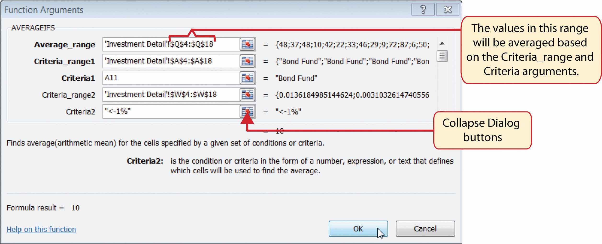
The AVERAGEIFS function will be used to calculate the average months of ownership for poor performing investments in the portfolio. The following steps explain how to add this function to the Portfolio Summary worksheet:
- Click cell C11 on the Portfolio Summary worksheet.
- Click the Formulas tab on the Ribbon.
- Click the More Functions button in the Function Library group of commands.
- Place the mouse pointer over the Statistical option from the drop-down list (see Figure 3.25 "Selecting the COUNTIF Function from the Function Library").
- Click the AVERAGEIFS function near the top of the list of functions. This will open the Function Arguments dialog box.
- Click the Collapse Dialog button next to the Average_range argument on the Function Arguments dialog box (see Figure 3.35 "Completed Arguments for the AVERAGEIFS Function").
- Click the Investment Detail worksheet tab.
- Highlight the range Q4:Q18 on the Investment Detail worksheet and press the ENTER key on your keyboard. Selected cells from this range will be averaged by the function based on the defined criteria in ensuing arguments.
- Click in the Average_range argument input box and place an absolute reference on the range Q4:Q18. This is done by typing a dollar sign ($) in front of the column letter and row number for both cells in the range.
- Click the Collapse Dialog button next to the Criteria_range1 argument on the Function Arguments dialog box (see Figure 3.35 "Completed Arguments for the AVERAGEIFS Function").
- Click the Investment Detail worksheet tab.
- Highlight the range A4:A18 on the Investment Detail worksheet and press the ENTER key on your keyboard. Once the Criteria_range1 argument is defined, the Criteria1 argument will appear in the Function Arguments dialog box.
- Click in the Criteria_range1 argument input box and place an absolute reference on the range A4:A18. This is done by typing a dollar sign ($) in front of the column letter and row number for both cells in the range.
- Press the TAB key on your keyboard to advance to the Criteria1 argument and type the cell location A11. The criteria for the function will be the investment type entered into cell A11 on the Portfolio Summary worksheet. You will notice that as you define this argument, the Criteria_range2 argument will appear on the Function Arguments dialog box.
- Click the Collapse Dialog button next to the Criteria_range2 argument on the Function Arguments dialog box (see Figure 3.35 "Completed Arguments for the AVERAGEIFS Function").
- Click the Investment Detail worksheet tab.
- Highlight the range W4:W18 on the Investment Detail worksheet and the press the ENTER key on your keyboard.
- Click in the Criteria_range2 argument input box and place an absolute reference on the range W4:W18. This is done by typing a dollar sign ($) in front of the column letter and row number for both cells in the range.
- Press the TAB key on your keyboard to advance to the Criteria2 argument.
- Type an open quotation mark followed by the logical test <−1% and then type a closing quotation mark (“<−1%”). The second criterion for this function is a logical test that will identify cell locations where the value is less than −1%. For the purposes of this exercise, a poor performing investment is one that is below the target growth rate by more than 1%.
- Click the OK button at the bottom of the Function Arguments dialog box.
-
Copy the function in cell C11 and paste it into the range C12:C14 using the Paste Formulas command.
Figure 3.35 "Completed Arguments for the AVERAGEIFS Function" shows the defined arguments for the AVERAGEIFS function. Notice that two sets of criteria arguments are defined. Values that meet all criteria defined in the function will be selected from the range Q4:Q18.
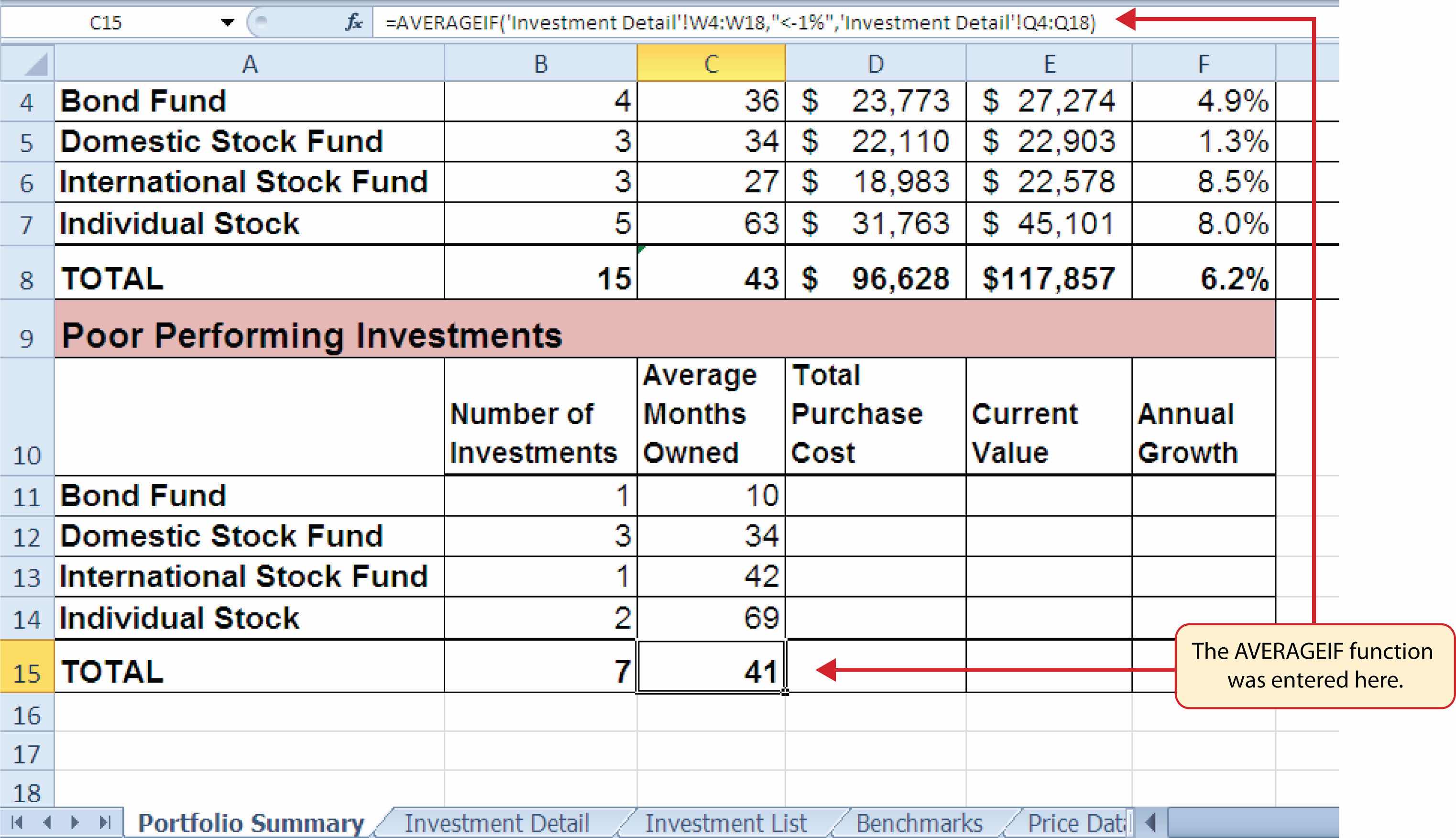
- Enter an AVERAGEIF function in cell C15 by typing an equal sign (=) followed by the function name AVERAGEIF followed by an open parenthesis (().
- Click the Investment Detail worksheet tab and highlight the range W4:W18 to define the Range argument. Type a comma.
- Type the following to define the criteria argument: “<–1%”. Type a comma.
- Highlight the range Q4:Q18 to define the [Average_range] argument. Then type a closing parenthesis ()) and press the ENTER key on your keyboard.
Figure 3.36 "Results of the AVERAGEIFS Function" shows the results of the AVERAGEIFS function in the Portfolio Summary worksheet. The function shows the average months of ownership for the poor performing investments by investment type.
Skill Refresher: AVERAGEIFS Function
- Type an equal sign (=).
- Type the function name AVERAGEIFS followed by an open parenthesis (().
- Define the Average_range argument with a range of cells that contain values to be averaged.
- Type a comma.
- Define the Criteria_range1 argument with a range of cells that will be evaluated based on the criteria used to define the Criteria1 argument.
- Type a comma.
- Define the Criteria1 argument with a cell location, number, text, or logical test. Text and logical tests must be enclosed in quotation marks.
- Repeat steps 4, 5, 6, and 7 to define as many pairs of criteria arguments as needed.
- Type a closing parenthesis ()).
- Press the ENTER key on your keyboard.
The SUMIFS Function
Follow-along file: Continue with Excel Objective 3.00. (Use file Excel Objective 3.13 if starting here.)
Lesson Video: SUMIFS Function
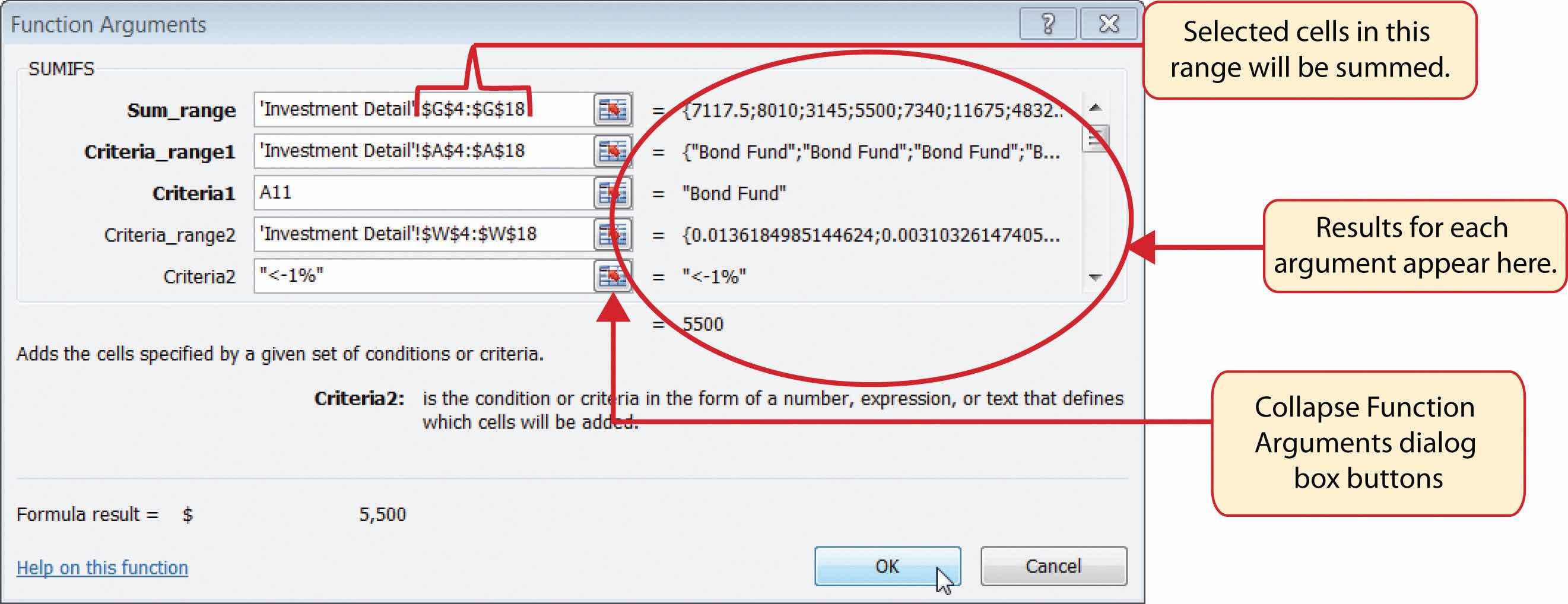
The SUMIFS function is similar to the AVERAGEIFS function in that multiple criteria arguments can be defined to select cells from a targeted range (see Table 3.9 "Arguments for the AVERAGEIFS and SUMIFS Functions"). The function will use the selected cells from this targeted range to calculate a total or sum. The SUMIFS function will be used to complete the Total Purchase Cost and Current Value columns in the Poor Performing Investments section of the Portfolio Summary worksheet. The following steps explain how to construct this function for the Total Purchase Cost column:
- Click cell D11 on the Portfolio Summary worksheet.
- Click the Formulas tab on the Ribbon.
- Click the Math & Trig button in the Function Library group of commands (see Figure 3.25 "Selecting the COUNTIF Function from the Function Library").
- Select the SUMIFS function from the drop-down list. Use the scroll bar to scroll down to find the SUMIFS function. This will open the Function Arguments dialog box.
- Click the Collapse Dialog button next to the Sum_range argument on the Function Arguments dialog box (see Figure 3.37 "Completed Arguments for the SUMIFS Function").
- Click the Investment Detail worksheet tab.
- Highlight the range G4:G18 on the Investment Detail worksheet and press the ENTER key on your keyboard. Selected cells from this range will be summed based on the defined criteria in ensuing arguments.
- Click in the Sum_range argument input box and place an absolute reference on the range G4:G18. This is done by typing a dollar sign ($) in front of the column letter and row number for both cells in the range.
- Click the Collapse Dialog button next to the Criteria_range1 argument on the Function Arguments dialog box (see Figure 3.37 "Completed Arguments for the SUMIFS Function").
- Click the Investment Detail worksheet tab.
- Highlight the range A4:A18 on the Investment Detail worksheet and press the ENTER key on your keyboard. Once the Criteria_range1 argument is defined, the Criteria1 argument will appear in the Function Arguments dialog box.
- Click in the Criteria_range1 argument input box and place an absolute reference on the range A4:A18. This is done by typing a dollar sign ($) in front of the column letter and row number for both cells in the range.
- Press the TAB key on your keyboard to advance to the Criteria1 argument and type the cell location A11. The criteria for the function will be the investment type that is entered into cell A11 on the Portfolio Summary worksheet. You will notice that as soon as you define this argument, the Criteria_range2 argument will appear on the Function Arguments dialog box.
- Click the Collapse Dialog button next to the Criteria_range2 argument on the Function Arguments dialog box (see Figure 3.37 "Completed Arguments for the SUMIFS Function").
- Click the Investment Detail worksheet tab.
- Highlight the range W4:W18 on the Investment Detail worksheet and press the ENTER key on your keyboard.
- Click in the Criteria_range2 argument input box and place an absolute reference on the range W4:W18. This is done by typing a dollar sign ($) in front of the column letter and row number for both cells in the range.
- Press the TAB key on your keyboard to advance to the Criteria2 argument.
- Type an open quotation mark followed by the logical test <−1% and then type a closing quotation mark (“<−1%”). The second criterion for this function is a logical test that will identify cell locations where the value is less than −1%. For the purposes of this exercise, a poor performing investment is one that is below the target growth rate by more than 1%.
- Click the OK button at the bottom of the Function Arguments dialog box.
- Copy the function in cell D11 and paste it into the range D12:D14 using the Paste Formulas command.
- Enter a regular SUM function in cell D15 on the Portfolio Summary worksheet that sums the values in the range D11:D14.
Figure 3.37 "Completed Arguments for the SUMIFS Function" shows the defined arguments for the SUMIFS function. Values that meet all criteria defined in the function will be selected from the range G4:G18. Notice that the results for each argument of the function are shown along the right side of the Collapse Dialog buttons.
Figure 3.38 "SUMIFS Function Output for the Total Purchase Cost Column" shows the results of the SUMIFS function used to complete the Total Purchase Cost column. In total, over $45,000 was invested in funds and stocks that are not meeting the performance goals of the portfolio.
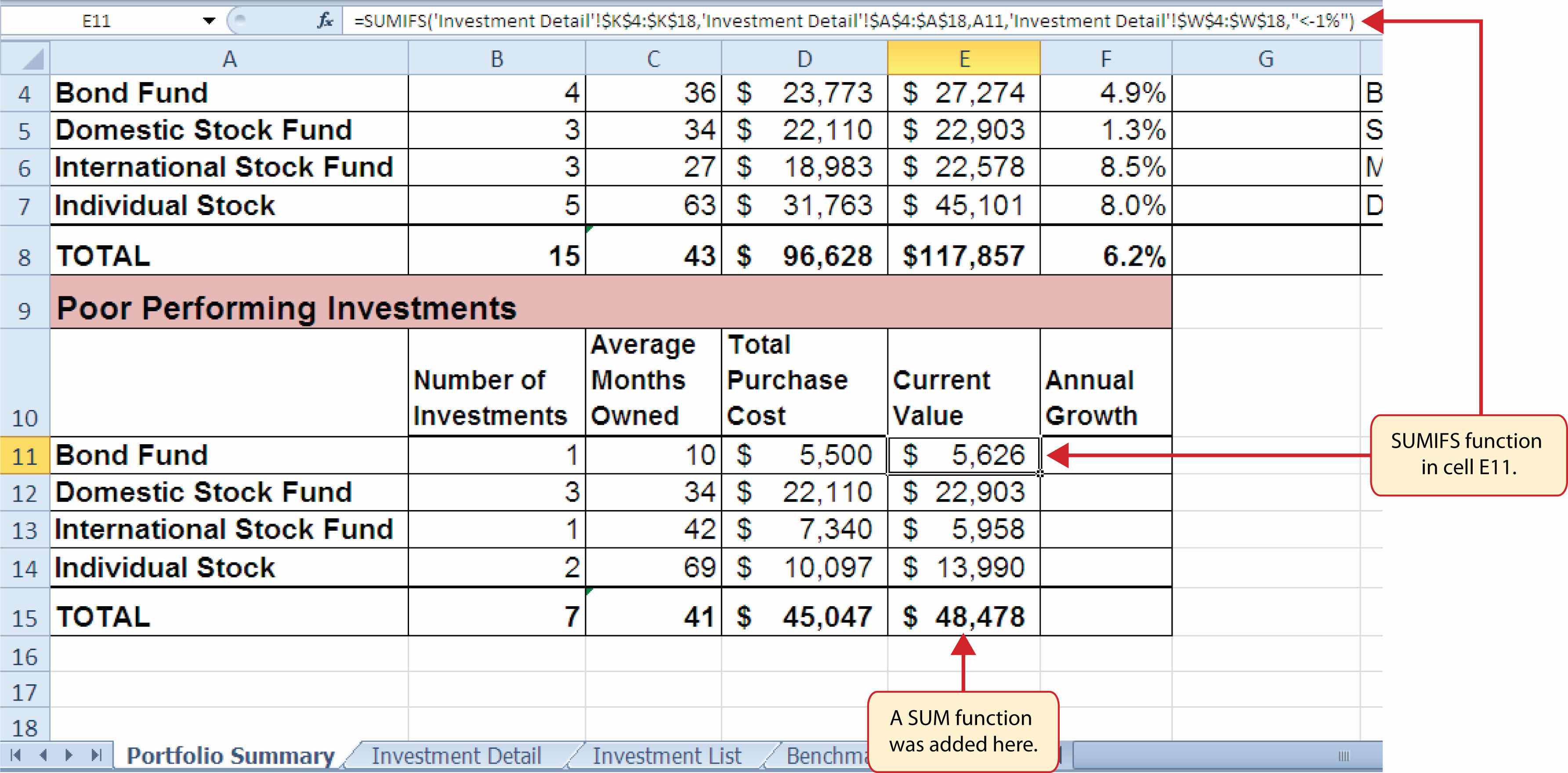
In addition to the Total Purchase Cost column, the SUMIFS function will also be used to complete the Current Value column for the Poor Performing Investments section on the Portfolio Summary worksheet. The following steps explain how to add the function to the worksheet to complete this column:
- Click cell E11 on the Portfolio Summary worksheet.
- Click the Formulas tab on the Ribbon.
- Click the Math & Trig button in the Function Library group of commands (see Figure 3.25 "Selecting the COUNTIF Function from the Function Library").
- Select the SUMIFS function from the drop-down list. Use the scroll bar to scroll down to find the SUMIFS function. This will open the Function Arguments dialog box.
- Click the Collapse Dialog button next to the Sum_range argument on the Function Arguments dialog box (see Figure 3.39 "Completed Function Arguments Dialog Box for the Second SUMIFS Function").
- Click the Investment Detail worksheet tab.
- Highlight the range K4:K18 on the Investment Detail worksheet and press the ENTER key on your keyboard. Selected cells from this range will be summed based on the defined criteria in ensuing arguments.
- Click in the Sum_range argument input box and place an absolute reference on the range K4:K18. This is done by typing a dollar sign ($) in front of the column letter and row number for both cells in the range.
- Click the Collapse Dialog button next to the Criteria_range1 argument on the Function Arguments dialog box (see Figure 3.39 "Completed Function Arguments Dialog Box for the Second SUMIFS Function").
- Click the Investment Detail worksheet tab.
- Highlight the range A4:A18 on the Investment Detail worksheet and press the ENTER key on your keyboard. Once the Criteria_range1 argument is defined, the Criteria1 argument will appear in the Function Arguments dialog box.
- Click in the Criteria_range1 argument input box and place an absolute reference on the range A4:A18. This is done by typing a dollar sign ($) in front of the column letter and row number for both cells in the range.
- Press the TAB key on your keyboard to advance to the Criteria1 argument and type the cell location A11. The criteria for the function will be the investment type entered into cell A11 on the Portfolio Summary worksheet.
- Click the Collapse Dialog button next to the Criteria_range2 argument on the Function Arguments dialog box (see Figure 3.39 "Completed Function Arguments Dialog Box for the Second SUMIFS Function").
- Click the Investment Detail worksheet tab.
- Highlight the range W4:W18 on the Investment Detail worksheet and press the ENTER key on your keyboard.
- Click in the Criteria_range2 argument input box and place an absolute reference on the range W4:W18. This is done by typing a dollar sign ($) in front of the column letter and row number for both cells in the range.
- Press the TAB key on your keyboard to advance to the Criteria2 argument.
- Type an open quotation mark followed by the logical test <−1% and then type a closing quotation mark (“<−1%”). The second criterion for this function is a logical test that will identify cell locations where the value is less than −1%. For the purposes of this exercise, a poor performing investment is one that is below the target growth rate by more than 1%.
- Click the OK button at the bottom of the Function Arguments dialog box.
- Copy the function in cell E11 and paste it into the range E12:E14 using the Paste Formulas command.
- Enter a regular SUM function in cell E15 on the Portfolio Summary worksheet that sums the values in the range E11:E14 (see Figure 3.40 "SUMIFS Function Output for the Current Value Column").
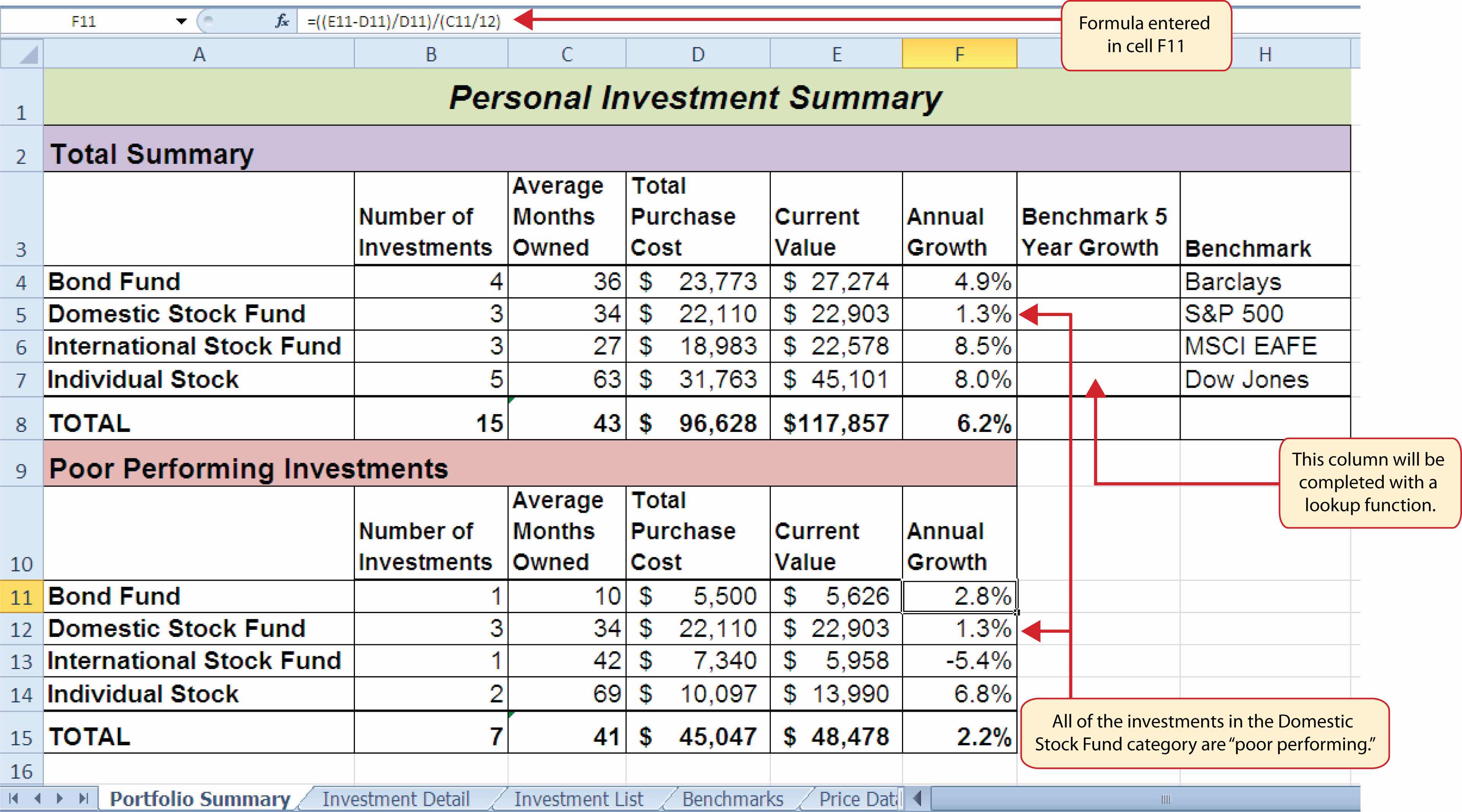
Now that the Total Purchase Cost and Current Value columns are completed for the Poor Performing Investments section on the Portfolio Summary worksheet, we can add a formula to show the annual growth rate by investment type. Since this is the same formula that was used in the Total Summary section of the Portfolio Summary worksheet, we can just copy and paste it. The following steps explain how to do this:
- Copy the formula in cell F4 on the Portfolio Summary worksheet.
- Highlight the range F11:F15 on the Portfolio Summary worksheet.
- Paste the formula using the Paste Formulas command.
Integrity Check
Error Message for Statistical IF Functions
If you receive an error message when attempting to enter a statistical IF function into a cell location, check to make sure any criteria using a comparison operator is enclosed in quotation marks. For example, if you are assessing a range of cells to see if the values are greater than or equal to zero, you must define the Criteria argument as follows: “>=0”. If you do not use the quotation marks, Excel will not accept the function in the cell location and will display an error message.
Figure 3.41 "Completed Poor Performing Investments Section of the Portfolio Summary Worksheet" shows the completed Poor Performing Investments section on the Portfolio Summary worksheet. Notice that even though an investment is considered “poor performing” it does not mean that money is lost on the investment. As shown in the figure, only one investment in the International Stock Fund category is losing money, with an annual growth rate of −5.4%. However, the total annual growth rate for all investments in the Poor Performing section is 2.2% (see cell F15). This is less than half the growth rate for the overall portfolio, which is 6.2% (see cell F8). A final observation is that all the investments in the Domestic Stock Fund category are “poor performing.” The same number of investments in the Total Summary section appears in the Poor Performing Investments section. This completes the Portfolio Summary worksheet with the exception of one column. We will complete this column in the next section with a lookup function.
Skill Refresher: SUMIFS Function
- Type an equal sign (=).
- Type the function name SUMIFS followed by an open parenthesis (().
- Define the Sum_range argument with a range of cells that contain values to be summed.
- Type a comma.
- Define the Criteria_range1 argument with a range of cells that will be evaluated based on the criteria used to define the Criteria1 argument.
- Type a comma.
- Define the Criteria1 argument with a cell location, number, text, or logical test. Text and logical tests must be enclosed in quotation marks.
- Repeat steps 4, 5, 6, and 7 to define as many pairs of criteria arguments as needed.
- Type a closing parenthesis ()).
- Press the ENTER key on your keyboard.
Key Takeaways
- The COUNTIF, SUMIF, and AVERAGEIF functions can select specific cell locations from a range to compute an output using one criteria argument.
- The COUNTIFS, SUMIFS, and AVERAGEIFS functions can select specific cell locations from a range to compute an output using multiple sets of criteria arguments.
- When using the AVERAGEIF and SUMIF functions, the row numbers used in the ranges to define the Range argument and the Average_range or Sum_range arguments must be identical.
- The benefit of using statistical functions when creating a summary worksheet is that if rows of data are added to the detail worksheet, the new data will automatically be included in the function output.
- When using statistical IF functions, the logical test used to define a criteria argument must be enclosed in quotation marks.
Exercises
-
Consider the following SUMIF function: =SUMIF(B2:B10,A1,E2:E20). What cell range will be used to compute the output for the function?
- E2:E10
- B2:B10
- E2:E20
- B2:B20
-
Which of the following is true with respect to the COUNTIF function?
- It can only be used to sum selected cells from a range using one set of defined criteria.
- It can be used to count both numeric and nonnumeric values in selected cells from a range using one set of defined criteria.
- It can be used to count only numeric values in selected cells from a range given one set of defined criteria.
- It can be used to count only numeric values in selected cells from a range using multiple sets of defined criteria.
-
If you wanted to calculate the average of the values contained in the range B5:B20 based on any values in the range E5:E20 with a value greater than 5, which of the following functions would provide an accurate result?
- =COUNTIF(B5:B20,>5,E5:E20)
- =AVERAGEIF(B5:B20,>5,E5:E20)
- =AVERAGEIF(E5:E20,>5,B5:B20)
- =AVERAGEIF(E5:E20,”>5”,B5:B20)
-
Suppose you wanted to sum the values in the range C3:C15 where the values in B3:B15 are equal to the word Bond and where the values in the range D3:D15 are greater than 3%. Which of the following functions would provide an accurate result?
- =SUMIFS(C3:C15,B3:B15,“Bond”,D3:D15,“>3%”)
- =SUMIFS(B3:B15,“Bond”,D3:D15,“>.03”,C3:C15)
- =SUMIFS($C$3:$C$15,$B$3:$B$15,“Bond”,$D$3:$D$15,>3%)
- =SUMIFS($B$3:$B$15,=Bond,$D$3:$D$15,>.03,$C$3:$C$1)