Acquiring geographic data is an important factor in any geographic information system (GIS) effort. It has been estimated that data acquisition typically consumes 60 to 80 percent of the time and money spent on any given project. Therefore, care must be taken to ensure that GIS projects remain mindful of their stated goals so the collection of spatial data proceeds in an efficient and effective manner as possible. This chapter outlines the many forms and sources of geospatial data available for use in a GIS.
The type of data that we employ to help us understand a given entity is determined by (1) what we are examining, (2) what we want to know about that entity, and (3) our ability to measure that entity at a desired scale. The most common types of data available for use in a GIS are alphanumeric strings, numbers, Boolean values, dates, and binaries.
An alphanumeric stringA data type made up of any simple combination of letters and numbers that may or may not form coherent words., or text, data type is any simple combination of letters and numbers that may or may not form coherent words. The number data type can be subcategorized as either floating-point or integer. A floating-pointA numerical data value that contains decimal digits. is any data value that contains decimal digits, while an integerA numerical data value that does not contain decimal digits. is any data value that does not contain decimal digits. Integers can be short or long depending on the amount of significant digits in that number. Also, they are based on the concept of the “bit” in a computer. As you may recall, a bit is the most basic unit of information in a computer and stores values in one of two states: 1 or 0. Therefore, an 8-bit attribute would consist of eight 1s or 0s in any combination (e.g., 10010011, 00011011, 11100111).
Short integersAn integer characterized by a 16-bit value. are 16-bit values and therefore can be used to characterize numbers ranging either from −32,768 to 32,767 or from 0 to 65,535 depending on whether the number is signed or unsigned (i.e., contains a + or − sign). Long integersAn integer characterized by a 32-bit value., alternatively, are 32-bit values and therefore can characterize numbers ranging either from −2,147,483,648 to 2,147,483,647 or from 0 to 4,294,967,295.
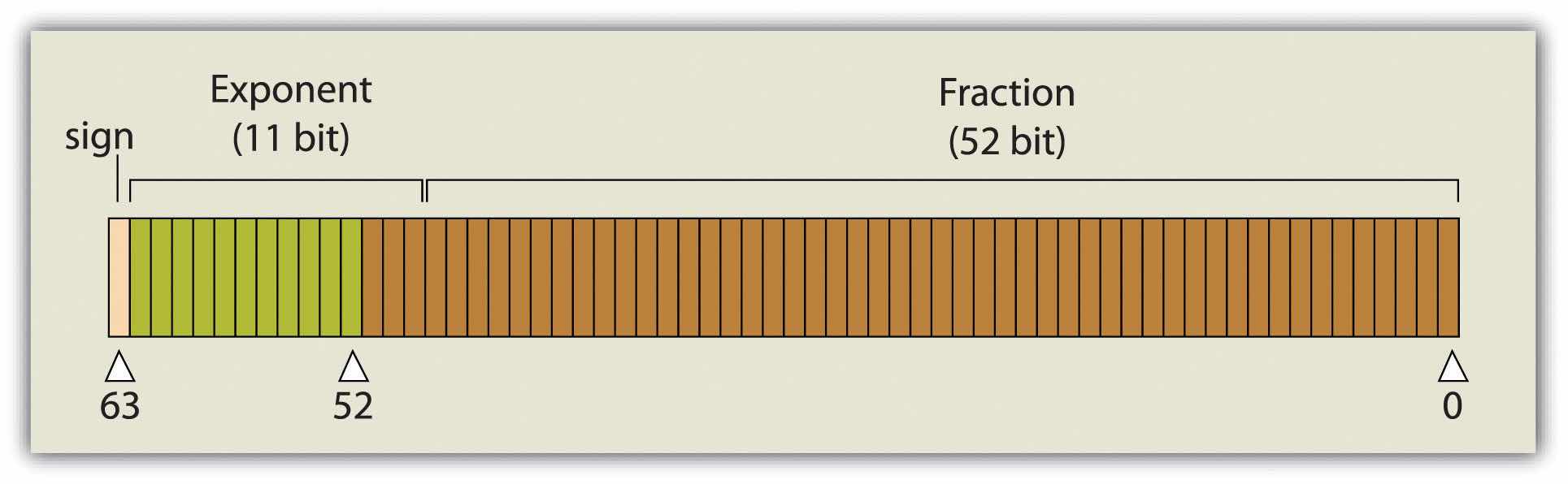
A single precision floating-pointA floating-point data value occupying 32 bits, characterized by up to 7 bits to the left of the decimal and up to 23 bit values to the right of the decimal point. value occupies 32 bits, like the long integer. However, this data type provides for a value of up to 7 bits to the left of the decimal (a maximum value of 128, or 127 if signed) and up to 23-bit values to the right of the decimal point (approximately 7 decimal digits). A double precision floating-pointA floating-point data value occupying 64 bits, characterized by up to 11 bits to the left of the decimal and up to 52 bit values to the right of the decimal point. value essentially stores two 32-bit values as a single value. Double precision floats, then, can represent a value with up to 11 bits to the left of the decimal point and values with up to 52 bits to the right of the decimal (approximately 16 decimal digits) (Figure 5.1 "Double Precision Floating-Point (64-Bit Value), as Stored in a Computer").
Figure 5.1 Double Precision Floating-Point (64-Bit Value), as Stored in a Computer
Boolean, date, and binary values are less complex. BooleanA data type whose values can be either true or false (1 or 0). values are simply those values that are deemed true or false based on the application of a Boolean operator such as AND, OR, and NOT. The date data type is presumably self-explanatory, while the binary data type represents attributes whose values are either 1 or 0.
In addition to defining data by type, a measurement scale acts to group data according to level of complexity (Stevens 1946).Stevens, S. S. 1946. “On the Theory of Scales of Measurement.” Science 103 (2684): 677–80. For the purposes of GIS analyses, measurement scales can be grouped in to two general categories. Nominal and ordinal data represent categorical data; interval and ratio data represent numeric data.
The most simple data measurement scale is the nominalA data scale that records the name of features but that does not allow for numerical, scalar comparisons between one object and another., or named, scale. The nominal scale makes statements about what to call data points but does not allow for scalar comparisons between one object and another. For example, the attribution of nominal information to a set of points that represent cities will describe whether the given locale is “Los Angeles” or “New York.” However, no further denotations, such as population or voting history, can be made about those locales. Other examples of nominal data include last name, eye color, land-use type, ethnicity, and gender.
Ordinal dataA data scale that places attribute information into ranks. places attribute information into ranks and therefore yields more precisely scaled information than nominal data. Ordinal data describes the position in which data occur, such as first, second, third, and so forth. These scales may also take on names, such as “very unsatisfied,” “unsatisfied,” “satisfied,” and “very satisfied.” Although this measurement scale indicates the ranking of each data point relative to other data points, the ordinal scale does not explicitly denote the exact quantitative difference between these rankings. For example, if an ordinal attribute represents which runner came in first, second, or third place, it does not state by how much time the winning runner beat the second place runner. Therefore, one cannot undertake arithmetic operations with ordinal data. Only sequence is explicit.
A measurement scale that does allow precise quantitative statements to be made about attributes is interval dataA data scale based on values with equal intervals but with no meaningful zero.. Interval data are measured along a scale in which each position is equidistant to one another. Elevation and temperature readings are common representations of interval data. For example, it can be determined through this scale that 30 ºF is 5 ºF warmer than 25 ºF. A notable property of the interval scale is that zero is not a meaningful value in the sense that zero does not represent nothingness, or the absence of a value. Indeed, 0 ºF does not indicate that no temperature exists. Similarly, an elevation of 0 feet does not indicate a lack of elevation; rather, it indicates mean sea level.
Ratio dataA data scale based on values with equal intervals and a meaningful zero. are similar to the interval measurement scale; however, it is based around a meaningful zero value. Population density is an example of ratio data whereby a 0 population density indicates that no people live in the area of interest. Similarly, the Kelvin temperature scale is a ratio scale as 0 K does imply that no heat (temperature) is measurable within the given attribute.
Specific to numeric datasets, data values also can be considered to be discrete or continuous. Discrete dataData that can are limited to a finite number of potential values. are those that maintain a finite number of possible values, while continuous dataData that can take on an infinite number of potential values. can be represented by an infinite number of values. For example, the number of mature trees on a small property will necessarily be between one and one hundred (for argument’s sake). However, the height of those trees represents a continuous data value as there are an infinite number of potential values (e.g., one tree may be 20 feet tall, 20.1 feet, or 20.15 feet, 20.157 feet, and so forth).
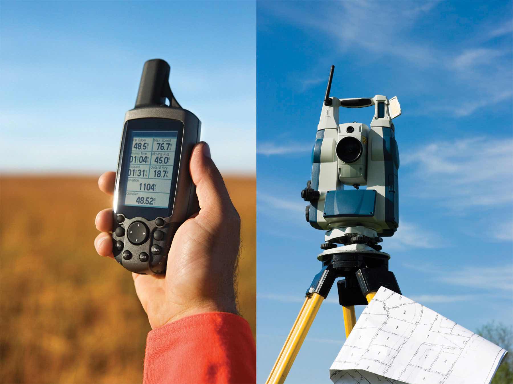
Now that we have a sense of the different data types and measurement scales available for use in a GIS, we must direct our thoughts to how this data can be acquired. Primary data captureA direct data acquisition methodology that is associated with an in-the-field effort. is a direct data acquisition methodology that is usually associated with some type of in-the-field effort. In the case of vector data, directly captured data commonly comes from a global positioning system (GPS) or other types of surveying equipment such as a total station (Figure 5.2 "GPS Unit (left) and Total Station (right)"). Total stations are specialized, primary data capture instruments that combine a theodolite (or transit), which measures horizontal and vertical angles, with a tool to measure the slope distance from the unit to an observed point. Use of a total station allows field crews to quickly and accurately derive the topography for a particular landscape.
Figure 5.2 GPS Unit (left) and Total Station (right)
In the case of GPS, handheld units access positional data from satellites and log the information for subsequent retrieval. A network of twenty-four navigation satellites is situated around the globe and provides precise coordinate information for any point on the earth’s surface (Figure 5.3 "Earth Imaging Satellite Capturing Primary Data"). Maintaining a line of sight to four or more of these satellites provides the user with reasonably accurate location information. These locations can be collected as individual points or can be linked together to form lines or polygons depending on user preference. Attribute data such as land-use type, telephone pole number, and river name can be simultaneously entered by the user. This location and attribute data can then be uploaded to the GIS for visualization. Depending on the GPS make and model, this upload often requires some type of intermediate file conversion via software provided by the manufacturer of the GPS unit. However, there are some free online resources that can convert GPS data from one format to another. GPSBabel is an example of such an online resource (http://www.gpsvisualizer.com/gpsbabel).
In addition to the typical GPS unit shown in Figure 5.2 "GPS Unit (left) and Total Station (right)", GPS is becoming increasingly incorporated into other new technologies. For example, smartphones now embed GPS capabilities as a standard technological component. These phone/GPS units maintain comparable accuracy to similarly priced stand-alone GPS units and are largely responsible for a renaissance in facilitating portable, real-time data capture and sharing to the masses. The ubiquity of this technology led to a proliferation of crowdsourced data acquisition alternatives. CrowdsourcingThe collection and reporting of spatial data by a diffuse user community. is a data collection method whereby users contribute freely to building spatial databases. This rapidly expanding methodology is utilized in such applications as TomTom’s MapShare application, Google Earth, Bing Maps, and ArcGIS.
Raster data obtained via direct capture comes more commonly from remotely sensed sources (Figure 5.3 "Earth Imaging Satellite Capturing Primary Data"). Remotely sensed data offers the advantage of obviating the need for physical access to the area being imaged. In addition, huge tracts of land can be characterized with little to no additional time and labor by the researcher. On the other hand, validation is required for remotely sensed data to ensure that the sensor is not only operating correctly but properly calibrated to collect the desired information. Satellites and aerial cameras provide the most ubiquitous sources of direct-capture raster data (Chapter 4 "Data Models for GIS", Section 4.3.1 "Satellite Imagery").
Figure 5.3 Earth Imaging Satellite Capturing Primary Data

Secondary data captureAn indirect data acquisition methodology that utilizes the vast amount of existing data available in both digital and hard-copy formats. is an indirect methodology that utilizes the vast amount of existing geospatial data available in both digital and hard-copy formats. Prior to initiating any GIS effort, it is always wise to mine online resources for existing GIS data that may fulfill your mapping needs without the potentially intensive step of creating the data from scratch. Such digital GIS data are available from a variety of sources including international agencies (CGIAR, CIESIN, United Nations, World Bank, etc.); federal governments (USGS, USDA, NOAA, USFWS, NASA, EPA, US Census, etc.); state governments (CDFG, Teale Data Center, INGIS, MARIS, NH GIS Resources, etc.); local governments (SANDAG, RCLIS, etc.); university websites (UCLA, Duke, Stanford, University of Chicago, Indiana Spatial Data Portal, etc.); and commercial websites (ESRI, GeoEye, Geocomm, etc.). These secondary data are available in a wide assortment of file types, extents, and sizes but is ready-made to be used in most GIS software packages. Often these data are free, but many sites will charge a fee for access to the proprietary information they have developed.
Although these data sources are all cases where the information has been converted to digital format and properly projected for use in a GIS, there is also a great deal of spatial information that can be gleaned from existing, nondigital sources. Paper maps, for example, may contain current or historic information on a locale that cannot be found in digital format. In this case, the process of digitizationThe conversion of analog information to digital information. can be used to create digital files from the original paper copy. Three primary methods exist for digitizing spatial information: two are manual, and one is automated.
Tablet digitizingA manual data capture method whereby a user enters coordinate information into a computer through the use of a digitizing tablet and a digitizing puck. is a manual data capture method whereby a user enters coordinate information into a computer through the use of a digitizing tablet and a digitizing puck. To begin, a paper map is secured to a back-lit digitizing tablet. The backlight allows all features on the map to be easily observed, which reduces eyestrain. The coordinates of the point, line, and/or polygon features on the paper map are then entered into a digital file as the user employs a puck, which is similar to a multibutton mouse with a crosshair, to “click” their way around the vertices of each desired feature. The resulting digital file will need to be properly georeferenced following completion of the digitization task to ensure that this information will properly align with existing datasets.
Heads-up digitizingA manual data capture method whereby a user traces the outlines of features on a computer screen., the second manual data capture method, is referred to as “on-screen” digitizing. Heads-up digitizing can be used on either paper maps or existing digital files. In the case of a paper map, the map must first be scanned into the computer at a high enough resolution that will allow all pertinent features to be resolved. Second, the now-digital image must be registered so the map will conform to an existing coordinate system. To do this, the user can enter control points on the screen and transform, or “rubber-sheet,” the scanned image into real world coordinates. Finally, the user simply zooms to specific areas on the map and traces the points, lines, and/or polygons, similar to the tablet digitization example. Heads-up digitizing is particularly simple when existing GIS files, satellite images, or aerial photographs are used as a baseline. For example, if a user plans to digitize the boundary of a lake as seen from a georeferenced satellite image, the steps of scanning and registering can be skipped, and projection information from the originating image can simply be copied over to the digitized file.
The third, automated method of secondary data capture requires the user to scan a paper map and vectorize the information therein. This vectorizationThe process of converting raster graphics to vector graphics. method typically requires a specific software package that can convert a raster scan to vector lines. This requires a very high-resolution, clean scan. If the image is not clean, all the imperfections on the map will likely be converted to false points/lines/polygons in the digital version. If a clean scan is not available, it is often faster to use a manual digitization methodology. Regardless, this method is much quicker than the aforementioned manual methods and may be the best option if multiple maps must be digitized and/or if time is a limiting factor. Often, a semiautomatic approach is employed whereby a map is scanned and vectorized, followed by a heads-up digitizing session to edit and repair any errors that occurred during automation.
The final secondary data capture method worth noting is the use of information from reports and documents. Via this method, one enters information from reports and documents into the attribute table of an existing, digital GIS file that contains all the pertinent points, lines, and polygons. For example, new information specific to census tracts may become available following a scientific study. The GIS user simply needs to download the existing GIS file of census tracts and begin entering the study’s report/document information directly into the attribute table. If the data tables are available digitally, the use of the “join” and “relate” functions in a GIS (Section 5.2.2 "Joins and Relates") are often extremely helpful as they will automate much of the data entry effort.
The following data are derived from which measurement scale?


