The raster data model is widely used in applications ranging far beyond geographic information systems (GISs). Most likely, you are already very familiar with this data model if you have any experience with digital photographs. The ubiquitous JPEG, BMP, and TIFF file formats (among others) are based on the raster data model (see Chapter 5 "Geospatial Data Management", Section 5.3 "File Formats"). Take a moment to view your favorite digital image. If you zoom deeply into the image, you will notice that it is composed of an array of tiny square pixels (or picture elements). Each of these uniquely colored pixels, when viewed as a whole, combines to form a coherent image (Figure 4.1 "Digital Picture with Zoomed Inset Showing Pixilation of Raster Image").
Figure 4.1 Digital Picture with Zoomed Inset Showing Pixilation of Raster Image

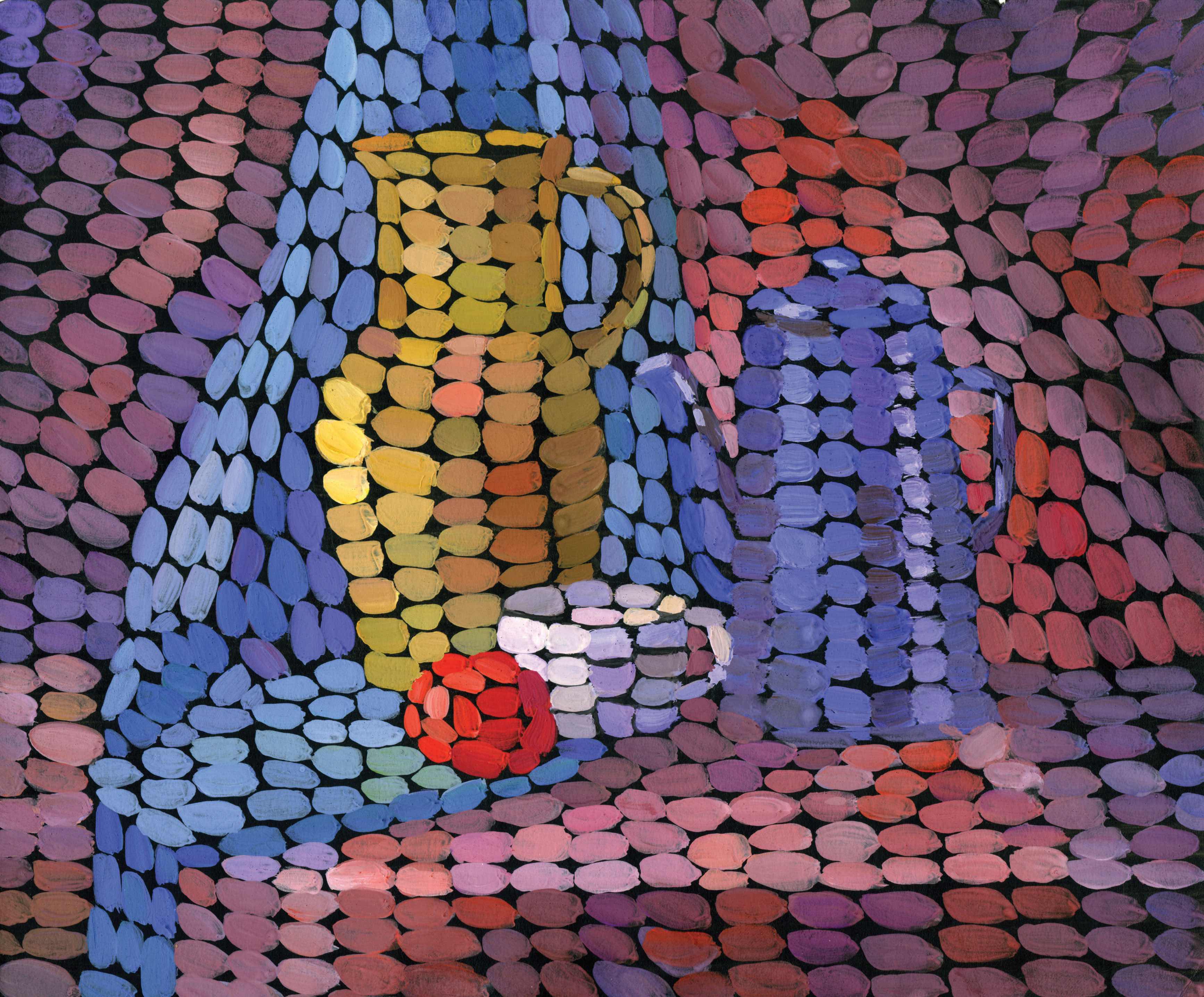
Furthermore, all liquid crystal display (LCD) computer monitors are based on raster technology as they are composed of a set number of rows and columns of pixels. Notably, the foundation of this technology predates computers and digital cameras by nearly a century. The neoimpressionist artist, Georges Seurat, developed a painting technique referred to as “pointillism” in the 1880s, which similarly relies on the amassing of small, monochromatic “dots” of ink that combine to form a larger image (Figure 4.2 "Pointillist Artwork"). If you are as generous as the author, you may indeed think of your raster dataset creations as sublime works of art.
Figure 4.2 Pointillist Artwork
The raster data model consists of rows and columns of equally sized pixels interconnected to form a planar surface. These pixels are used as building blocks for creating points, lines, areas, networks, and surfaces (Chapter 2 "Map Anatomy", Figure 2.6 "Map Overlay Process" illustrates how a land parcel can be converted to a raster representation). Although pixels may be triangles, hexagons, or even octagons, square pixels represent the simplest geometric form with which to work. Accordingly, the vast majority of available raster GIS data are built on the square pixel (Figure 4.3 "Common Raster Graphics Used in GIS Applications: Aerial Photograph (left) and USGS DEM (right)"). These squares are typically reformed into rectangles of various dimensions if the data model is transformed from one projection to another (e.g., from State Plane coordinates to UTM [Universal Transverse Mercator] coordinates).
Figure 4.3 Common Raster Graphics Used in GIS Applications: Aerial Photograph (left) and USGS DEM (right)
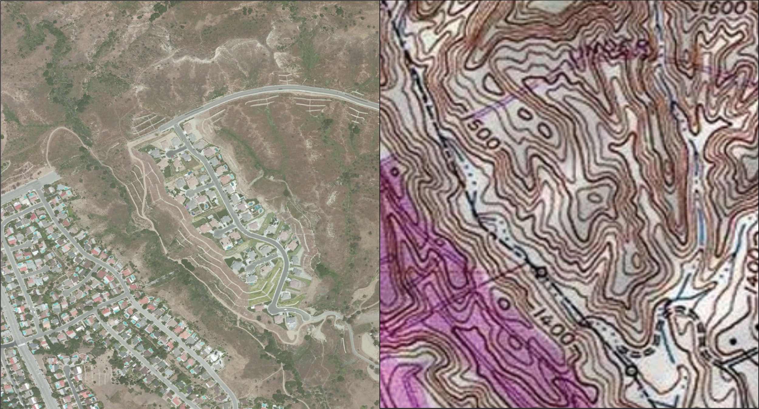
Source: Data available from U.S. Geological Survey, Earth Resources Observation and Science (EROS) Center, Sioux Falls, SD.
Because of the reliance on a uniform series of square pixels, the raster data model is referred to as a grid-based system. Typically, a single data value will be assigned to each grid locale. Each cell in a raster carries a single value, which represents the characteristic of the spatial phenomenon at a location denoted by its row and column. The data type for that cell value can be either integer or floating-point (Chapter 5 "Geospatial Data Management", Section 5.1 "Geographic Data Acquisition"). Alternatively, the raster graphic can reference a database management system wherein open-ended attribute tables can be used to associate multiple data values to each pixel. The advance of computer technology has made this second methodology increasingly feasible as large datasets are no longer constrained by computer storage issues as they were previously.
The raster model will average all values within a given pixel to yield a single value. Therefore, the more area covered per pixel, the less accurate the associated data values. The area covered by each pixel determines the spatial resolutionThe smallest distance between two adjacent features that can be detected in an image. of the raster model from which it is derived. Specifically, resolution is determined by measuring one side of the square pixel. A raster model with pixels representing 10 m by 10 m (or 100 square meters) in the real world would be said to have a spatial resolution of 10 m; a raster model with pixels measuring 1 km by 1 km (1 square kilometer) in the real world would be said to have a spatial resolution of 1 km; and so forth.
Care must be taken when determining the resolution of a raster because using an overly coarse pixel resolution will cause a loss of information, whereas using overly fine pixel resolution will result in significant increases in file size and computer processing requirements during display and/or analysis. An effective pixel resolution will take both the map scale and the minimum mapping unit of the other GIS data into consideration. In the case of raster graphics with coarse spatial resolution, the data values associated with specific locations are not necessarily explicit in the raster data model. For example, if the location of telephone poles were mapped on a coarse raster graphic, it would be clear that the entire cell would not be filled by the pole. Rather, the pole would be assumed to be located somewhere within that cell (typically at the center).
Imagery employing the raster data model must exhibit several properties. First, each pixel must hold at least one value, even if that data value is zero. Furthermore, if no data are present for a given pixel, a data value placeholder must be assigned to this grid cell. Often, an arbitrary, readily identifiable value (e.g., −9999) will be assigned to pixels for which there is no data value. Second, a cell can hold any alphanumeric index that represents an attribute. In the case of quantitative datasets, attribute assignation is fairly straightforward. For example, if a raster image denotes elevation, the data values for each pixel would be some indication of elevation, usually in feet or meters. In the case of qualitative datasets, data values are indices that necessarily refer to some predetermined translational rule. In the case of a land-use/land-cover raster graphic, the following rule may be applied: 1 = grassland, 2 = agricultural, 3 = disturbed, and so forth (Figure 4.4 "Land-Use/Land-Cover Raster Image"). The third property of the raster data model is that points and lines “move” to the center of the cell. As one might expect, if a 1 km resolution raster image contains a river or stream, the location of the actual waterway within the “river” pixel will be unclear. Therefore, there is a general assumption that all zero-dimensional (point) and one-dimensional (line) features will be located toward the center of the cell. As a corollary, the minimum width for any line feature must necessarily be one cell regardless of the actual width of the feature. If it is not, the feature will not be represented in the image and will therefore be assumed to be absent.
Figure 4.4 Land-Use/Land-Cover Raster Image
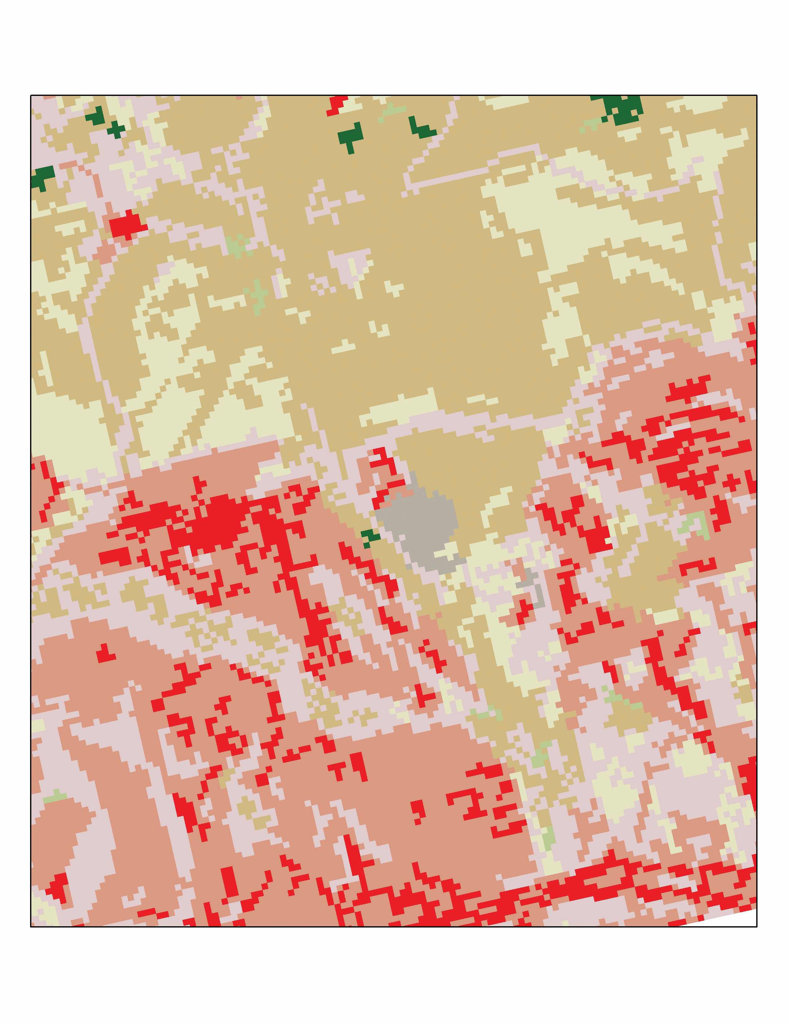
Source: Data available from U.S. Geological Survey, Earth Resources Observation and Science (EROS) Center, Sioux Falls, SD.
Several methods exist for encoding raster data from scratch. Three of these models are as follows:
Figure 4.5 Cell-by-Cell Encoding of Raster Data
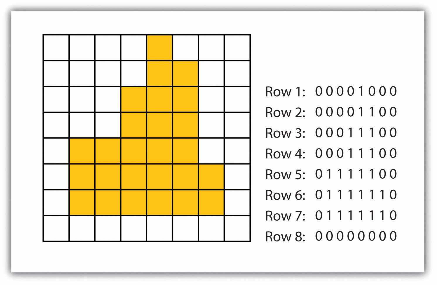
Figure 4.6 Run-Length Encoding of Raster Data
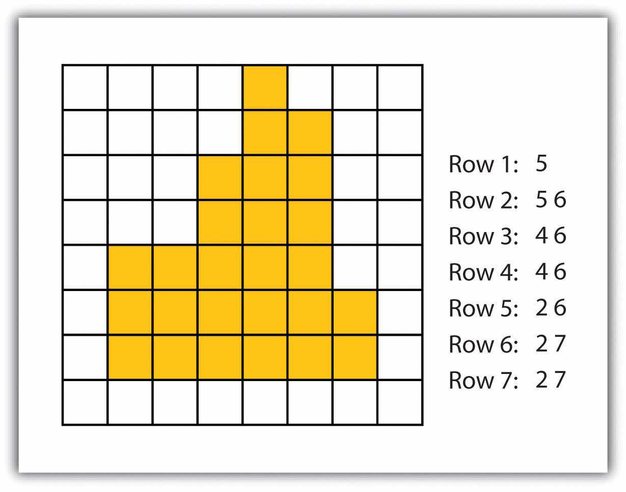
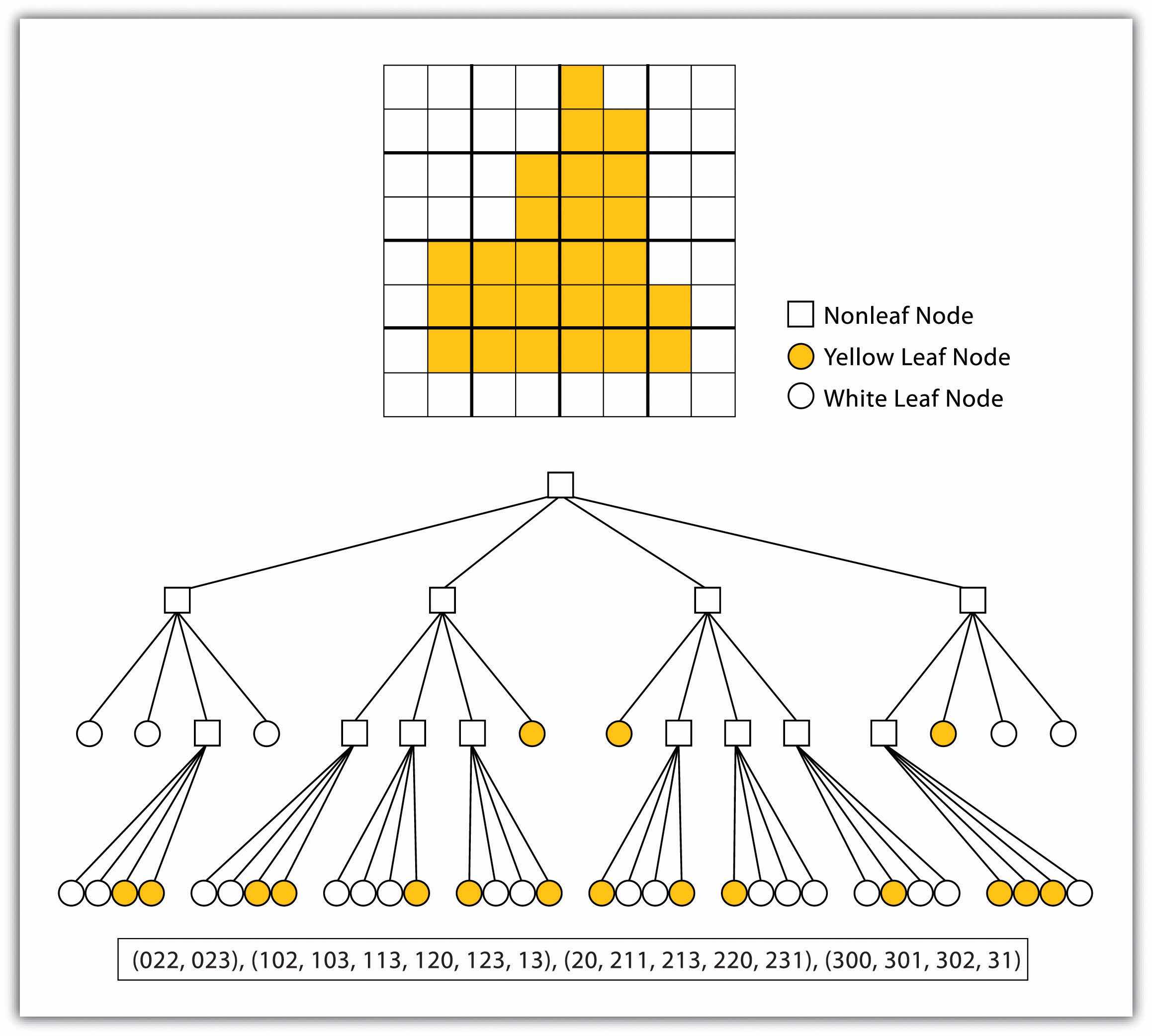
Figure 4.7 Quad-Tree Encoding of Raster Data
The use of a raster data model confers many advantages. First, the technology required to create raster graphics is inexpensive and ubiquitous. Nearly everyone currently owns some sort of raster image generator, namely a digital camera, and few cellular phones are sold today that don’t include such functionality. Similarly, a plethora of satellites are constantly beaming up-to-the-minute raster graphics to scientific facilities across the globe (Chapter 5 "Geospatial Data Management", Section 5.3 "File Formats"). These graphics are often posted online for private and/or public use, occasionally at no cost to the user.
Additional advantages of raster graphics are the relative simplicity of the underlying data structure. Each grid location represented in the raster image correlates to a single value (or series of values if attributes tables are included). This simple data structure may also help explain why it is relatively easy to perform overlay analyses on raster data (for more on overlay analyses, see Chapter 7 "Geospatial Analysis I: Vector Operations", Section 7.1 "Single Layer Analysis"). This simplicity also lends itself to easy interpretation and maintenance of the graphics, relative to its vector counterpart.
Despite the advantages, there are also several disadvantages to using the raster data model. The first disadvantage is that raster files are typically very large. Particularly in the case of raster images built from the cell-by-cell encoding methodology, the sheer number of values stored for a given dataset result in potentially enormous files. Any raster file that covers a large area and has somewhat finely resolved pixels will quickly reach hundreds of megabytes in size or more. These large files are only getting larger as the quantity and quality of raster datasets continues to keep pace with quantity and quality of computer resources and raster data collectors (e.g., digital cameras, satellites).
A second disadvantage of the raster model is that the output images are less “pretty” than their vector counterparts. This is particularly noticeable when the raster images are enlarged or zoomed (refer to Figure 4.1 "Digital Picture with Zoomed Inset Showing Pixilation of Raster Image"). Depending on how far one zooms into a raster image, the details and coherence of that image will quickly be lost amid a pixilated sea of seemingly randomly colored grid cells.
The geometric transformations that arise during map reprojection efforts can cause problems for raster graphics and represent a third disadvantage to using the raster data model. As described in Chapter 2 "Map Anatomy", Section 2.2 "Map Scale, Coordinate Systems, and Map Projections", changing map projections will alter the size and shape of the original input layer and frequently result in the loss or addition of pixels (White 2006).White, D. 2006. “Display of Pixel Loss and Replication in Reprojecting Raster Data from the Sinusoidal Projection.” Geocarto International 21 (2): 19–22. These alterations will result in the perfect square pixels of the input layer taking on some alternate rhomboidal dimensions. However, the problem is larger than a simple reformation of the square pixel. Indeed, the reprojection of a raster image dataset from one projection to another brings change to pixel values that may, in turn, significantly alter the output information (Seong 2003).Seong, J. C. 2003. “Modeling the Accuracy of Image Data Reprojection.” International Journal of Remote Sensing 24 (11): 2309–21.
The final disadvantage of using the raster data model is that it is not suitable for some types of spatial analyses. For example, difficulties arise when attempting to overlay and analyze multiple raster graphics produced at differing scales and pixel resolutions. Combining information from a raster image with 10 m spatial resolution with a raster image with 1 km spatial resolution will most likely produce nonsensical output information as the scales of analysis are far too disparate to result in meaningful and/or interpretable conclusions. In addition, some network and spatial analyses (i.e., determining directionality or geocoding) can be problematic to perform on raster data.


