Process-Oriented Design

3. Definition of Structured Design Terms

TABLE 8 - 1 Structured Design Concept Definitions

Term	Definition
Stepwise refinement	The process of defining functions that will accomplish a process; includes definition of modules, programs, and data
Program morphology	The shape of a program, including the extent of fan-out, fan-in, scope of control, and scope of effect
Data structure	The definition of data in an application includes logical data definition and physical data structure
Modularity	A property of programs meaning they are divided into several separate addressable elements
Abstraction	Attention to some level of g~neralization without regard to irrelevant lowlevel details
Information hiding	Design decisions in one module are hidden from other modules
Cohesion	A measure of the internal strength of a module
Coupling	A measure of the intermodule strength ofa module

The streams are partitioned off from the rest of the diagram by drawing arcs showing where they end.
Examples of transform-centered applications include accounting, personnel, payroll, or order entry-inventory control. For these applications, getting data into and out of the system is secondary to the file handling and manipulation of numbers that keep track of the information. In accounting, for instance, balancing of debits and credits takes place at end-of-day, end-of-month, and end-of-year processing. These periodic process transformations summarize and move data, erase some information, archive other information, and write data to the general ledger to summarize the details in the receivables and payables subledgers. All of these transforms process data that is already in the files.
These processes are the heart of accounting processing. Without these processes, the application would be doing something else.
Not all applications are transform-centered. Some applications do simple processing but have many different transaction types on which the simple processes are performed. These systems are called transaction-centered. Transaction analysis replaces transform analysis for transaction-centered applications with partitioning by transaction type, which may not be obvious from DFDs. Figure 8-3 shows an example of a partitioned DFD for a transaction-centered application. This detailed DFD looks like it contains redundancy because many of the same processes appear more than once. Look closely and you see that each set of processes relates to a different type of transaction.
When the high-level partitioning is done, the information is transferred to a first-cut structure chart. We will develop the structure chart from Figure 8-2. A structure chart is a hierarchic, input process-output view of the application that reflects the DFD partitioning. The structure chart contains one rectangle for each lowest level process on the DFD. The rectangles are arranged in a hierarchy to show superior control and coordination modules. Individual process modules are the lowest in their hierarchy. The rectangles in the hierarchy are connected via undirected lines that are always read topdown and left to right. The lines imply transfer of processing from the top to the bottom of the hierarchy. Diamonds overlay the connection when a conditional execution of a module is possible using if-then-else logic. Reused modules are shown in one of two ways. Either they are repeated several times on the diagram and have a slash in the lower left corner to signify reuse, or they are connected to more than one superior module via the linking lines.
The identification of afferent flows, efferent flows, and transforms results in chains of processes, each its own 'net output.' If we look at Figure 8-2 again, we see the net afferent output is data flow Good Input. For the central transform, the net output is Solution. For the efferent flows, the net output is Printed Solution. These net outputs are used to determine the initial structure of the structure chart, using a process called factoring.

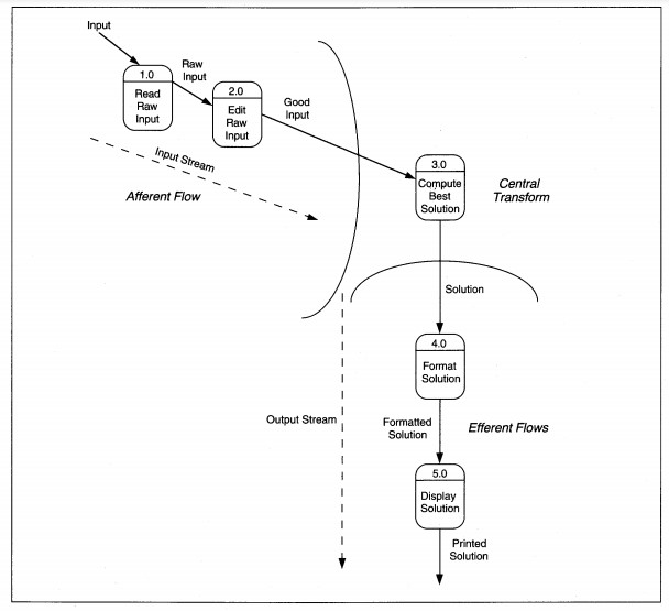
FIGURE 8-2 Transform-Centered DFD Partitioned

Factoring is the process of decomposing a DFD into a hierarchy of program components that will eventually be programmed modules, functions, or control structures. Each stream of processing is analyzed to determine its IPO structure. When the structure is identified, the processes are placed on the structure chart and named until all low-level DFD processes are on the structure chart (see Figure 8-4).

Next, data and control information are added to the structure chart. Data couples identify the flow of data into and out of modules and match the data flows on the DFD. Data couples are identified by a directed arrow with an open circle at the source end (see Figure 8-5). The arrowhead points in the direction the data moves. Control couples identify the flow of control in the structure. Control couples are placed to show where the control data originates and which module(s) each couple affects. A control couple is usually a program switch whose value identifies how a module is activated.

Control couples are drawn as directed arrows with a closed circle at the source end (see Figure 8-6). The arrowhead points in the direction the control travels. If a control couple is in, set and reset in the same module, it is not shown on the diagram. A control couple that is set and reset in one place, but used in another, is shown. If a control couple is set in one module and reset in another, it is shown as both input and output. Control is 'designed into' the application by you, the SE, based on the need for one module to control the processing of another module. The goal is to keep control to a minimum. Figure 8-4 shows the completed structure chart for the DFD in Figure 8-2.

Next, we evaluate and revise the structure chart to balance its morphology. Morphology means form or shape. The shape of the structure chart should be balanced to avoid processing bottlenecks. Balance is determined by analyzing the depth and width of the hierarchy, the skew of modules, the span of control, the scope of effect, and the levels of coupling and cohesion. When one portion of the structure chart is unbalanced in relation to the rest of the diagram, you modify the structure to restore the balance, or pay closer attention to the unbalanced portion to ensure an efficient production environment.

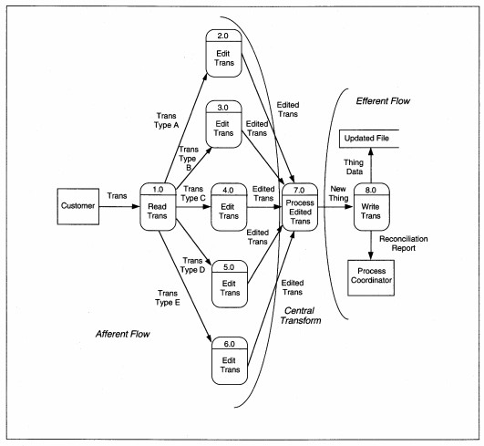
FIGURE 8-3 Transaction-Centered DFD Partitioned

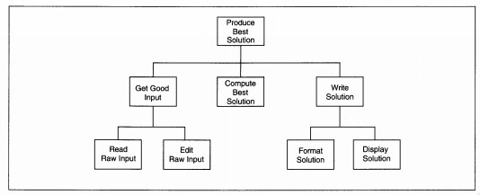
FIGURE 8-4 First-Cut Structure Chart

The depth of a hierarchy is the number of levels in the diagram. Depth by itself is not a measure of good design nor is it a goal in itself. Rather, it can indicate the problem of too much communication overhead and not enough real work taking place (see Figure 8-7). Conversely, adding a level of depth can be a cure for too wide a hierarchy.

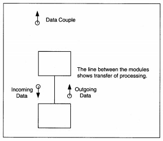
FIGURE 8-5 Data Couple Notation

The width of the hierarchy is a count of the modules directly reporting to each superior, higher level module (see Figure 8-8). Span of control is another term for the number of immediate subordinates and is a synonym for the width of the hierarchy. Width relates to two other terms: fanout and fan-in. Fan-out is the number of immediate subordinate modules. Too much fan-out can identify a processing bottleneck because a superior module is controlling too much processing.

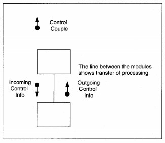
FIGURE 8-6 Control Couple Notation

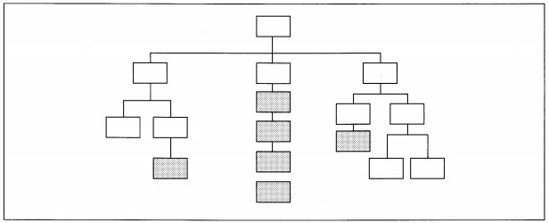
FIGURE 8-7 Excessive Depth of Hierarchy

While there is no one number that says 'how wide is too wide,' seven ±2 is the generally accepted guideline for number of fan-out modules. One solution to fan-out processes that are functionally related is to factor another level of processing that provides middle-level management of the low-level modules. Another solution to fan-out problems that are factored properly, but not functionally related, is to introduce a new control module at the IPO level.

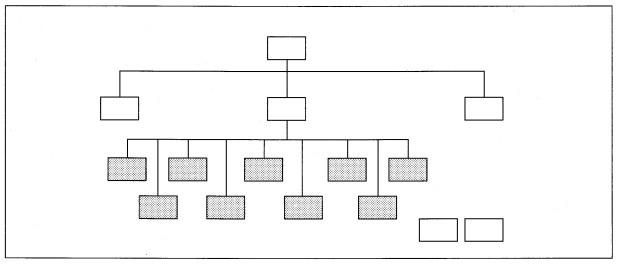
FIGURE 8-8 Excessive Width of Hierarchy

Fan-in, on the other hand, is the number of superior modules (i.e., immediate bosses) which refer to some subordinate module (see Figure 8-9). Fan-in can be desirable when it identifies reusable components and reduces the total amount of code produced. The major tasks with fan-in modules are to ensure that they perform a whole task, are highly cohesive, and are minimally coupled.

Skew is a measure of balance or lopsidedness of the structure chart (see Figure 8-10). Skew occurs when one high-level module has many subordinate levels and some or most of the other high-level modules have few subordinate levels. Skew can indicate incorrect factoring. If factoring is correct, then skew identifies a driver for the application that might require special consideration. If the skew is on the input side, we say the application is input driven or input-bound. Similarly, if the skew is on the output side, the application is output-bound. If the input and output are skewed with little transform processing, the application is I/O-bound (for input/output). Finally, if the application has little input or output, but lots of processing, the application is processbound. The special considerations of each of these occurrences deal with ensuring correct language selection and meeting I/O and process time constraints.

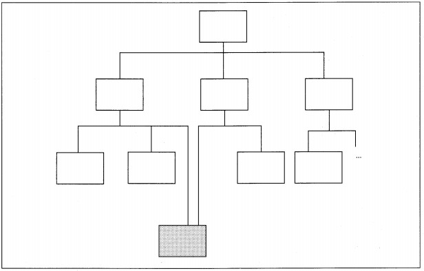
FIGURE 8-9 Example of Fan-In

The scope of effect of a module identifies the collection of modules that are conditionally processed based on decisions by that module (see Figure 8-11). The scope of effect can be identified by counting the number of modules that are directly affected by the process results of another module. High scope of effect relates to fan-out, fan-in, and coupling in that it may identify potential problems with debugging and change management. Ideally, the scope of effect of anyone module should be zero or one. That is, no more than one other module should be affected by any processing that takes place in any other module.

The last measures of structure morphology which are analyzed throughout the remainder of structure design are coupling and cohesion. Cohesion is a measure of the intramodule strength. Coupling is a measure of the intermodule linkage. Maximal, functional cohesion and minimal coupling are the ideal relationships. Coupling and cohesion are related inversely (see Figure 8-12). If cohesion is high, coupling is low, and vice versa; but, the relationship is not perfect. That means that if you have strong cohesion, you may still have strong coupling due to poor design. So, attention to both coupling and cohesion are required.

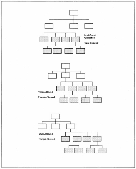
FIGURE 8-10 Examples of Skewed Structure Charts

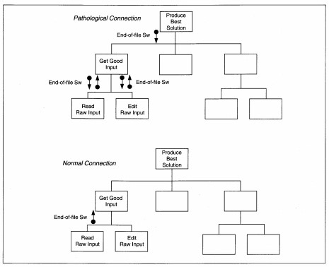
FIGURE 8-11 Example of Scope of Effect

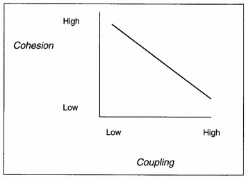
FIGURE 8- 12 Relationship between Coupling and Cohesion

Factoring and evaluation are followed by functional decomposition, which is the further division of processes into self-contained IPO subprocesses. Balanced structure chart subprocesses might be further decomposed to specify all of the functions required to accomplish each subprocess. Fan-out, span of control, and excessive depth are to be avoided during this process. 1 The decision whether to decompose further or not relates to the details needed for the implementation language and how well the SEs understand the details.

Structure charts are only one of many methods and techniques for documenting structured design results. Most of the alternatives would replace, rather than supplement, structure charts. Each technique has its own slightly different way of thinking about the processes to finalize a design, even though the goals are the same. Several alternatives are IBM Hierarchic input-process-output diagrams (HIPO) (see Figure 8-13), Warnier diagrams (see Figure 8-14), Nassi-Schneiderl11an diagrams (see Figure 8-15), and flow charts (see Figure 8-16).

To complete design, program specifications (specifications is abbreviated to 'specs') must be developed, but before specs can be developed, several other major activities are required. First, the physical database must be designed. Then, program package units are decided. Several activities not discussed here (these are covered in Chapter 14) are performed, including verification of adequate design for inputs, outputs, screens, reports, conversion, controls, and recoverability.

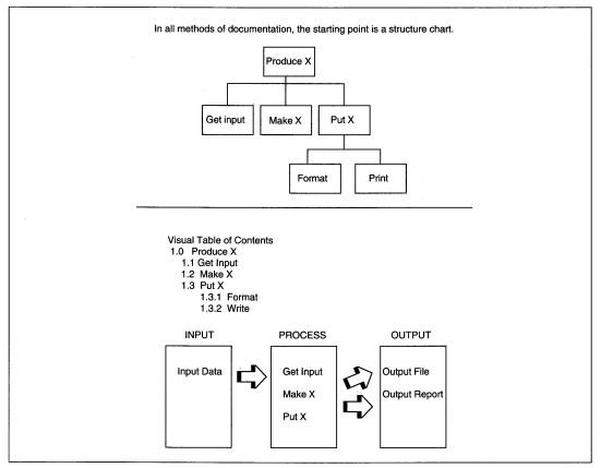
FIGURE 8- 13 Other Structured Program Documentation Methods: IBM's Hierarchic InputProcess-Output (HIPO) Diagram Example

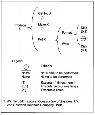
FIGURE 8-14 Warnier Diagram¹

Physical database design is concurrent with factoring and decomposition. Several common physical database design activities are:

design user views (if this is not already done)
select the access method
map user views to the access method and storage media
walk-through the database design
prototype the database
document and distribute access information to all team members
train team members in access requirements
develop a test database
develop the production database

Keep in mind that many other activities may be involved in designing a physical database for a specific implementation environment.

While the details of physical database design and decomposition are being finalized, project team members are also thinking about how to package the modules into program units. A program unit or a program package is one or more called modules, functions, and in-line code that will be an execute unit to perform some atomic process. In nonrealtime languages, an execute unit is a link-edited load module. In real-time languages, an execute unit identifies modules that can reside in memory at the same time and are closely related, usually by mutual communication. The guiding principles during these design activities are to minimize coupling and maximize cohesion (see Tables 8-2 and 8-3 for definition of the seven levels of coupling and cohesion).

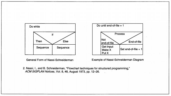
FIGURE 8-15 Nassi-Schneiderman2 Diagram Example

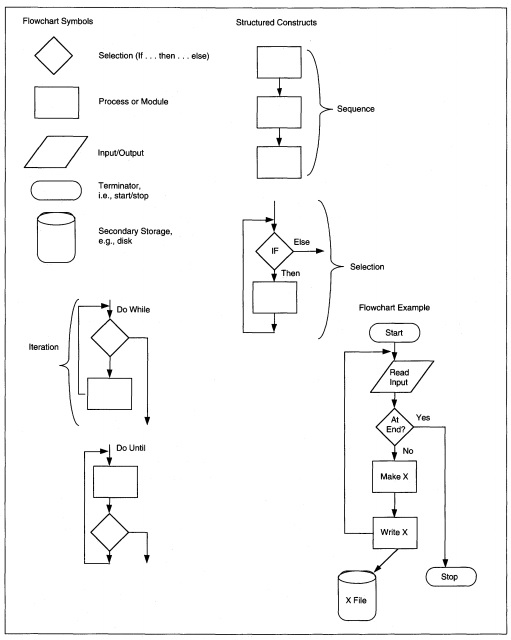
FIGURE 8-16 Flowchart Symbols, Structured Constructs, and Example

An atomic process is a system process that cannot be further decomposed without losing its systemlike qualities. An execute unit is a computer's unit of work (i.e., a task). A module is a 'small program' that is self-contained and may call other modules. Modules may be in-line, that is, in the actual program, or may be externally called modules. In-line code is the structured program code that controls and sequences execution of modules and functions. For instance, a 'read' module might do all file access; a screen interaction module might do all screen processing and have submodules that perform screen input and screen output.

A function is an external 'small program' that is self-contained and performs a well-defined, limited procedure. For example, a function might compute a square root of a number. Functions usually do not call other modules but there is no rule against it. Even though the definitions of modules and functions are similar, they are different entities. Functions sometimes come with a language, for instance, the mathematical and statistical functions that are part of Fortran. Modules are usually user-defined and have a broader range of applicability, such as a screen interaction module. Functions are usually reusable across applications without alteration; modules are not.

TABLE 8-2 Definition of Cohesion Levels

Type of Cohesion	Definition
Functional	Elements of a procedure are combined because they are all required to complete one specific function. This is the strongest type of cohesion and is the goal.
Sequential	Elements of a common procedure are combined because they are in the same procedure and data flows from one step to the next. That is, the output of one module, for example, is passed in sequence as input to the next module. This is a strong form of cohesion and is acceptable.
Communicational	Elements of a procedure are combined because they all use the same data type. Modules that all relate to customer maintenance-add, delete, update, query-are related through communication because they all use the Customer File.
Procedural	Elements of a common procedure are combined because they are in the same procedure and control flows from one step to the next. This is weak cohesion because passing of control does not mean functions in the procedure are related.
Temporal	Statements are together because they occur at the same time. This usually refers to program modules, for example, 'housekeeping' in COBOL programs to initialize variables, open files, and prepare for processing. Temporal cohesion is weak and should be avoided wherever practical.
Logical	The elements of a module are grouped by their type of function. For instance, all edits, all reads from files, or all input operations are grouped. This is undesirable cohesion and should be avoided.
Coincidental	This is the random or accidental placement of functions. This lowest level of cohesion occurs when there is no real relationship between elements of a module. This is undesirable cohesion and should be avoided.

TABLE 8-3 Definition of Coupling Levels

Level of Coupling	Definition
Indirect relationship	No coupling is possible when modules are independent of each other and have neither a need nor a way to communicate. This is desirable when modules are independent. An example of no direct relationship is a date translate routine and a net present value routine. There is no reason for them to be related, so they should not be related.
Data	Only necessary data are passed between two modules. There are no redundant parameters or data items. This is the desirable form of coupling for related modules.
Stamp	The module is given access to a complete data structure such as a physical data record when it only needs one or two items. The module becomes unnecessarily dependent on the format and arrangement of data items in the structure. Usually, stamp coupling implies external coupling. The presence of unneeded data violates the principal of 'information hiding' which says that only data needed to perform a task should be available to the task.
Control	Control 'flags' are shared across modules. Control coupling is normal if the setting and resetting of the flag are done by the same module. It is a pathological connection to be avoided if practical when one module sets the flag and the other module resets the flag.
External	Two modules reference the same data item or group of items such as a physical data record. In traditional batch applications, external coupling is unavoidable since data are passive and not directly relating to modules. External coupling is to be minimized as much as possible and avoided whenever practical. External coupling violates the principal of information hiding.
Common	Modules have access to data through global or common data areas. This is frequently a language construct problem but it can be avoided by passing parameters with only a small amount of additional work. Common coupling violates the principal of information hiding.
Content	One module directly references and/or changes the insides of another module or when normal linkage mechanisms are bypassed. This is the highest level of coupling and is to be avoided.

When program packages are decided, program interprogram relationships is interface. specifications are developed. Program specifications document the program's purpose, process requirements, the logical and physical data definitions, input and output formats, screen layouts, constraints, and special processing considerations that might complicate the program. Keep in mind that the term program might also mean a module within a program or an externally called function. There are two parts to a program specification: one identifies interprogram (including programs in other applications) relationships and communication; the other documents intraprogram processing that takes place within the individual program. Another term for interprogram relationships is interface.