Excel Formulas

Page 1

Our spreadsheet

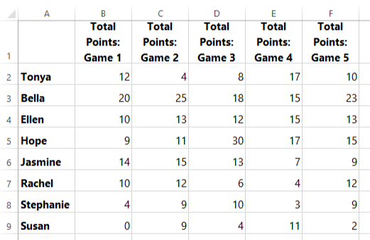
Once you've downloaded our spreadsheet, open the file in Excel or another spreadsheet application. You may want to take a moment to see how the data is organized. As you can see, there is a different row for each of the players and different columns for the number of points they scored in each game.

What are we trying to figure out?

Before we write our formulas, let's think about the problem we're trying to solve. Our friend wants to find out which player scored the most points total over these five games.

Writing the formula

Now that we know what function to use, we'll start by calculating the total points scored for Tonya in row 2.

Before we write the formula, we'll need to decide what cell range to include in the argument.

Now we're ready to write our formula. Go to the next page to see our formula in action!

Page 2

Writing the formula

Now that we know what function and cell range to use, we're ready to enter our formula, =SUM(B2:F2), in cell G2:

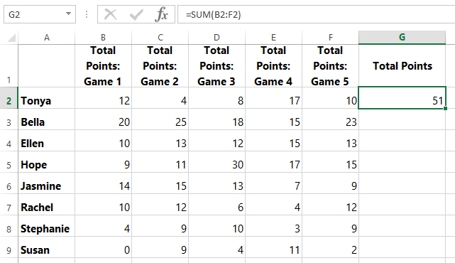
It looks like Tonya scored 51 points total. Next, we'll drag the fill handle down to add this formula for the other players.

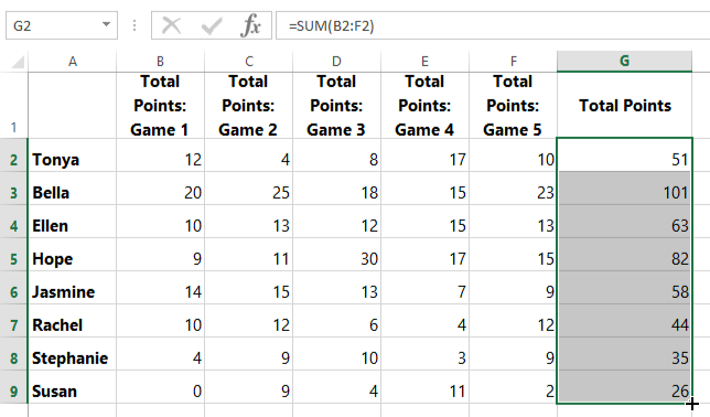
There we go! It looks like Bella scored the most points overall. However, we could take it a bit further to make our data really stand out. For example, we could:

• Apply conditional formatting to highlight the highest values
• Create a chart to visually compare the results
• Sort the results

There's really no right answer in this case—the most important thing is to make your data clear and easier to understand. In this example, it might be especially helpful to sort the data by the total points scored from highest to lowest—this will show who the top scorer is and make it easier to rank the other players on the team. Sorting works a bit differently, depending on which spreadsheet program you're using:

• For Excel 2007-2013: Select column G, then click the Descending Sort (Z-A) command on the Data tab.
  
• For Excel 2003 and earlier: Select column G, then click DataSortDescending.
• For Google Sheets: Select column G, then click DataSort Sheet by column GDescending.

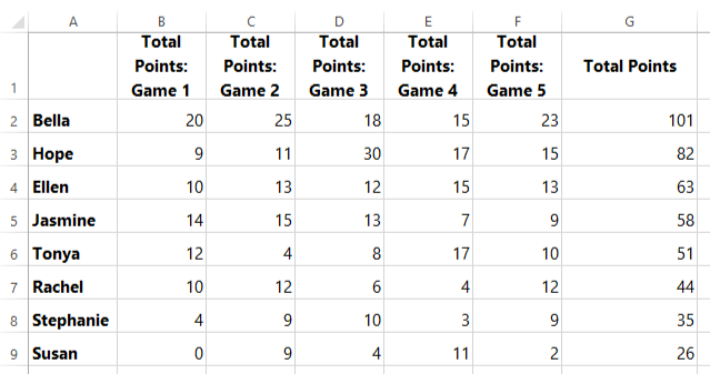
OK, now it's really easy to read our results! We can tell at a glance that Bella is the highest scorer, and we can also rank the other players.

Highest-scoring game for each player

Now we'll need to answer this question: How many points did each of the players score in their best-scoring game?

Now that we know what function to use, we'll start by finding the highest-scoring game for Bella in row 2.

Before we write our formula, we'll need to decide what cell range to include in the argument.

Go to the next page to see our formula in action!

Page 3

Highest-scoring game

Now that we know what function and cell range to use, we'll type our formula, =MAX(B2:F2), in cell H2 and then use the fill handle to add it to the other cells in column H.

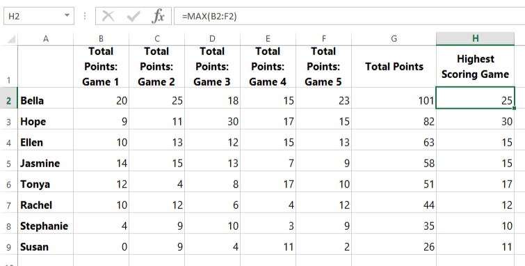
Now we can easily see how many points each of the players scored in their highest-scoring game!