Excel 2007: Formatting Tables

Page 1

Introduction

Formatting Tables Once you have entered information into a spreadsheet, you may want to format it. Formatting your spreadsheet can not only make it look nicer but also easier to use. In a previous lesson, we discussed manual formatting options such as bold and italics. In this lesson, you will learn how to use the predefined tables styles in Excel 2007 and some of the Table Tools on the Design tab.

Page 2

Formatting tables

Watch the video! (3:45 min)

To format information as a table:

Select any cell that contains information.
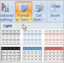
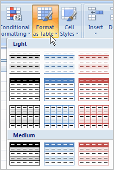
Click the Format as Table command in the Styles group on the Home tab. A list of predefined tables will appear.

Left-click a table style to select it.
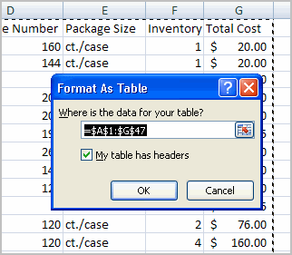
A dialog box will appear. Excel has automatically selected the cells for your table. The cells will appear selected in the spreadsheet, and the range will appear in the dialog box.

Change the range listed in the field if necessary.
Verify that the box is selected to indicate your table has headings, if it does. Deselect this box if your table does not have column headings.
Click OK. The table will appear formatted in the style you chose.

By default, the table will be set up with the drop-down arrows in the header so you can filter the table if you wish.

In addition to using the Format as Table command, you can select the Insert tab and click the Table command to insert a table.

Page 3

To modify a table:

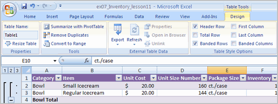
Select any cell in the table. The Table Tools Design tab will become active. From here, you can modify the table in several ways.

You can:

Select a different table in the Table Styles Options group. Click the More drop-down arrow to see more table styles.
Delete or add a Header Row in the Table Styles Options group.
Insert a Total Row in the Table Styles Options group.
Remove or add banded rows or columns.
Make the first and last columns bold.
Name your table in the Properties group.
Change the cells that make up the table by clicking Resize Table.

When you apply a table style, filtering arrows automatically appear. To turn off filtering, select the Home tab, click the Sort & Filter command, and select Filter from the list.

Page 4

Challenge!

Use the Inventory workbook or any workbook you choose to complete this challenge.

Format the information in a worksheet as a table.
Format the first column in bold.
Name the table.
Change the table style.
Practice using the other features discussed in this lesson to modify the table in various ways.