
Excel 2007
Formatting Text
Introduction
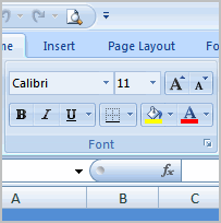 Once you have entered information into a spreadsheet, you will need to be able to format it. In this lesson, you will learn how to use the bold, italic, and underline commands; modify the font style, size, and color; and apply borders and fill colors.
Formatting cells
Watch the video! (8:32 min.)
Download the example to work along with the video.
To format text in bold or italics:
- Left-click a cell to select it, or drag your cursor over the text in the formula bar to select it.
- Click the Bold or Italics command.
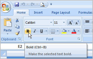
You can select entire columns and rows, or specific cells. To select the entire column, just left-click the column heading, and the entire column will appear as selected. To select specific cells, just left-click a cell and drag your mouse to select the other cells, then release the mouse button.
To format text as underlined:
- Select the cell or cells you want to format.
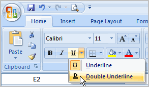
- Click the drop-down arrow next to the Underline command.
- Select the Single Underline or Double Underline option.
To change the font style
- Select the cell or cells you want to format.
- Left-click the drop-down arrow next to the Font Style box on the Home tab.
- Select a font style from the list.
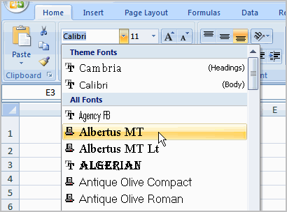
As you move over the font list, the Live Preview feature previews the font for you in the spreadsheet.
To change the font size:
- Select the cell or cells you want to format.
- Left-click the drop-down arrow next to the Font Size box on the Home tab.
- Select a font size from the list.
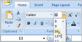
To change the text color:
- Select the cell or cells you want to format.
- Left-click the drop-down arrow next to the Text Color command. A color palette will appear.
- Select a color from the palette.
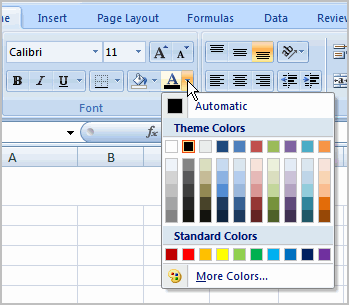
OR
- Select More Colors. A dialog box will appear.
- Select a color.
- Click OK.
To add a border:
- Select the cell or cells you want to format.
- Click the drop-down arrow next to the Borders command on the Home tab. A menu will appear with border options.
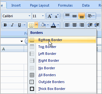
- Left-click an option from the list to select it.
You can change the line style and color of the border.
To add a fill color:
- Select the cell or cells you want to format.
- Click the Fill command. A color palette will appear.
- Select a color.
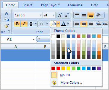
OR
- Select More Colors. A dialog box will appear.
- Select a color.
- Click OK.
You can use the fill color feature to format columns and rows and format a worksheet so it's easier to read.
To format numbers and dates:
- Select the cell or cells you want to format.
- Left-click the drop-down arrow next to the Number Format box.
- Select one of the options for formatting numbers.
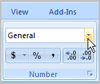
By default, the numbers appear in the General category, which means there is no special formatting.
In the Number group, you have some other options. For example, you can change the U.S. dollar sign to another currency format, switch numbers to percents, add commas, and change the decimal location.
Challenge!
Use the Budget workbook or any Excel workbook you choose to complete this challenge.
- Select a cell, then format the text or numbers in it so they appear bolded.
- Select two or more cells, and format the text or numbers so they appear in italics.
- Change fill color of two or more cells.
- Add a border to a row.