Excel 2000

Introduction

By the end of this lesson, learners should be able to:

• Create complex formulas
• Fill a formula to another cell
• Copy and paste a formula to another cell
• Revise a formula
• Create an absolute reference

Complex Formulas

Simple formulas have one mathematical operation. Complex formulas involve more than one mathematical operation.

The order of mathematical operations is very important. If you enter a formula that contains several operations, like adding, subtracting and dividing, Excel knows to work those operations in a specific order. The order of operations is:

1. Operations enclosed in parenthesis
2. Exponential calculations (to the power of)
3. Multiplication and division, whichever comes first
4. Addition and subtraction, whichever comes first

Relative to the order, you will also calculate from left to right. Let's look at an example.

2*(6-4) =?

Is the answer 8 or 4? If you calculated in the order in which the numbers appear, ignoring the parentheses, 2*6-4, you'd get the wrong answer, 8. You must follow the order of operations to get the correct answer.

To Calculate the Correct Answer,

1. Calculate the operation in parenthesis 6-4=2.
2. Multiply 2*2=4.
3. The answer is 4.

When using formulas, the results change each time the numbers are edited.

Remember: In Excel, never do math "in your head" and type the answer in a cell where you would expect to have a formula calculate the answer.

Creating Complex Formulas

When you create a complex formula, Excel automatically follows the order of operations. So, if you want a certain portion of the formula to be calculated first, put it in parentheses. For example, =(B8+B9)*A10.

1. Enter the numbers you want to calculate.
2. Click the cell where you want the formula result to appear.
3. Type =.
4. Click on the first cell to be included in the formula. The reference displays where you want your result.
5. Type a mathematical operator (Ex: the addition symbol +). The operator displays in the cell and Formula bar.
6. Click on the second cell in the formula. The reference displays where you want your result.
7. Type the next operator in the formula. The operator displays in the cell and Formula bar.
8. Click on the third cell to be included in the formula. The reference displays where you want your result.
9. Repeat steps 7 and 8 until the formula is complete, adding parentheses where necessary.
10. Very Important: Press Enter or click the Enter button on the Formula bar. This step ends the formula.

Try changing one of the values in the formula and watch the answer to the formula change.

Excel will not always tell you if your formula contains an error, so it's up to you to check all of your formulas. To learn how to do this, read the Double-Check Your Formulas lesson from our Excel Formulas tutorial.

Filling Formulas

Once you've created a working formula, don't waste time typing it over and over again. Simply fill it to the other cells. In order to do this, you will need to recognize the mouse pointer's various shapes. When you move the mouse pointer around the Excel window, it changes shape and function.

If you're going to copy a formula to a surrounding cell, you can use the Fill method. The square box in the lower right corner of the cell pointer is the fill handle.



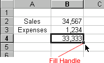
To Use the Fill Handle:

• Click on the cell that contains the formula.
• Position the mouse pointer on the lower right corner of the beginning of the cell pointer (fill handle). The mouse pointer becomes a black crosshair.
• Click and hold the left mouse button and drag to select the next cells to be filled in. The cells are now selected.
• Release the mouse button. The formula is copied.

In Excel, the references change as the formula is copied. (Remember, you use references to identify cells containing the numbers you want to calculate in a formula.)

You can also use copy and paste to copy a formula to other cells. Click next to learn more about the copy and paste method.

Copying and Pasting Formulas

While you can use both the fill method and the copy and paste method to copy a formula to surrounding cells, if you want to copy a formula to cells beyond the cells adjacent to the formula, use copy and paste.

To Use Copy and Paste:

• Select the cell with the formula you want to copy.
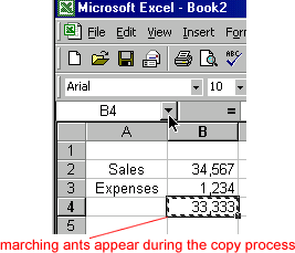
• Click the Copy button. Marching "ants" appear around the copied cells.
• Click the area where you want to place the duplicated formula.
• Press the Enter key. The formula is copied to the new location.

Cut, Copy, and Paste are discussed in detail in the Office 2000 lessons.

Revising Formulas

If you entered an incorrect formula or added new data and need to change the formula to reflect the new entries, you can revise your formula using the Range Finder or your keyboard.

What is the Range Finder?

• Double-click the cell that contains the formula you want to edit.
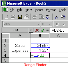
• Excel colors each cell address or range address in the formula a different color. (Below, see B4.)
• Corresponding colored borders appear around the cell or range. Each colored border is called a Range Finder. (Below, see B2 and B3.) This makes it easy to see whether a formula refers to the correct cells.

To Revise a Formula using the Range Finder:

• Select the cell or range you want to revise, and drag its Range Finder (the mouse pointer should be an arrow) to the cell or range with which you want to replace it. (Below, see Figure 1.)
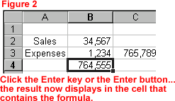
• Press the Enter key or click the Enter button to complete the formula.
• The new result now displays in the cell that contains the formula. (Below, see Figure 2.)

To Revise using the Keyboard:

• Double-click the cell that contains the formula you want to revise. The Range Finder displays.
• Select the cell or range you want to revise.
• Select another cell or range with which you want to replace it.
• Press the Enter key or click the Enter button. The result now displays in the cell that contains the formula.

You can also select the cell that contains the formula, select the part of the formula you want to revise, and type a new cell address. This is a somewhat inaccurate method, as it's easy to mistype.

Absolute References

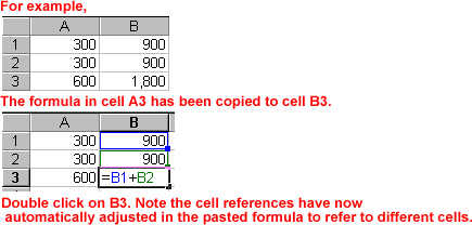
Normally, when you copy a formula that uses references, Excel automatically adjusts the reference in the pasted formula to refer to different cells relative to the position of the formula.

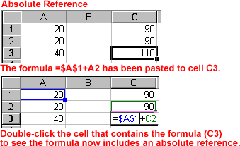
Sometimes, when you copy a formula, you don't want one of the cell references to change. Creating an Absolute reference, a reference to a cell that does not change when copying a formula, solves this problem. An absolute reference always refers to the same cell or range. It is designated in the formula by the dollar sign ($).

For this exercise, delete the original formulas and start again.

To Delete a Formula:

• Select the cells in which the original formulas exist. The cells are now selected.
• Press the Delete key. The information in these cells is deleted.

To Create an Absolute Reference:

• Enter the numbers you want to calculate. Then, create a simple formula (=A1+A2).
• Click on the cell in which you want to place the formula answer.
• To create an absolute reference, add a dollar sign ($) in front of the column reference and the row reference (=$A$1+A2).
• Press the Enter key or click the Enter button. The answer displays in the cell.
• Copy and Paste the formula to another adjacent cell. The formula now includes an absolute reference (=$A$1+C2).

Did You Know?

Knowing the Order of Operations is absolutely essential to getting the correct answer. Spend some time memorizing it:

1. Operations enclosed in parenthesis
2. Exponential calculations (to the power of)
3. Multiplication and division, whichever comes first
4. Addition and subtraction, whichever comes first